


Introduction
Most of us are familiar with the union-find data structure and the two optimizations one can do on it: union by rank and path compression. Most tutorials will introduce these methods and state that if both optimizations are used, the complexity will be $$$\mathcal{O}((n + m) \alpha(n))$$$. Here, $$$n$$$ and $$$m$$$ are the number of vertices and queries respectively. What is $$$\alpha$$$? Generally, we are told that $$$\alpha$$$ is some mysterious function that grows very slowly: $$$\alpha(N) < 5$$$ where $$$N$$$ is the number of subsets of particles in the observable universe and whatnot. What it is is usually not clarified very much. And there is typically no proof (or intuition and other such justifications) as to why the complexity is like that: usually we're told that the complexity analysis is quite long and complicated. At the time of writing, both cp-algorithms and Wikipedia are like that.
After telling students more or less the same thing for the $$$N$$$-th time, I finally decided to actually delve into the proof and see what is so difficult about it. My main motivation was to find out:
- How does one even analyze the time complexity of path compression — it seems quite chaotic?
- How does the Ackermann function of all things show up here? Why is it related to finding connected components or shortening paths on a tree?
In this blog, I will show the proof first published in Efficiency of a Good But Not Linear Set Union Algorithm by R. E. Tarjan, published in Journal of the ACM, Volume 22, Issue 2 in 1975. I will attempt to give a reader-friendly exposition of Tarjan's proof. Besides proving an upper bound on the complexity of the union-find data structure, in the article a lower bound is also calculated. I will not delve into the latter proof in this blog. In addition to the article, I decided to add examples of how to calculate worse upper bounds, because the techniques involved are similar and I believe it gives a better understanding of the ideas if we don't immediately jump to the hardest case.
Having read the proof, I believe it is not at all very long and complicated. Although it must've taken serious brainpower to come up with the techniques involved, the proof itself is a perfectly sensible chain of reasoning. The proof appears to be roughly 4 pages long at first glance, but 1 page of it is spent on the case without union-by-rank and 1 page is spent on listing various properties of the Ackermann function. The actual proof is therefore about 2 pages long, which I would consider short (the pages seem to be A5 with a rather large font). Furthermore, it is elementary: it's not one of those things that you can only understand if you have taken 3 semesters of algebraic topology. I can of course understand why this proof is not usually given in DSU lectures: knowing the proof is not particularly useful for solving problems and other very slow-growing upper bounds can be derived easily. But at least I think the difficulty of the argument should not be an excuse.
Prerequisites: comfortable with union-find and math. $$$~$$$
Recap: union-find and path compression
This will be brief because this is not a union-find tutorial. I will just quickly recount the definitions so we will be on the same page.
Disjoint set union (DSU) or union-find is a data structure that solves the following problem:
You are given a graph with $$$n$$$ vertices and initially no edges. You are given $$$m$$$ queries of the following type:
- "Union" (or "merge" or "unite"): given two vertices $$$u$$$ and $$$v$$$, add an edge between them.
- "Find": given a vertex $$$u$$$, find a representative of the connected component $$$u$$$ is in. This method should return the same value for any vertex in that connected component.
The problem is solved using the following data structure: we maintain a forest, where every connected component is represented as a tree. The "find" queries can be answered by moving from the vertex to the root of the tree; the "union" queries can be performed by setting the root of one tree as the parent to the root of the other tree.
// in initialization, parent[w] is set to w for every w
int find (int u) {
    if (parent[u] != u) {
        return find(parent[u]);
    }
    return u;
}

void merge (int u, int v) {
    u = find(u);
    v = find(v);
    parent[u] = v;
}
Path compression. Path compression is the following optimization to DSU:
int find (int u) {
    if (parent[u] != u) {
        parent[u] = find(parent[u]);
    }
    return parent[u];
}
After a query to find(u), for all vertices that used to be on the path from $$$u$$$ to the current root of the tree $$$u$$$ is in, their parent will be set to the current root of the tree.
Union-by-rank and its complexity
The analysis of the algorithm makes heavy use of ranks, so I put this part in a separate section.
Rank of a vertex. The rank of a vertex in a forest is the height of its subtree. Leaves have rank 0, vertices whose all children are leaves have rank 1 and so on.
Union-by-rank. Union by rank is the following optimization to DSU: when merging two trees, the root which has higher rank will be set as the parent to the other root. We will dynamically maintain the rank of each vertex. In code, it looks like this:
// in initialization, rank[w] is set to 0 for every w
void merge (int u, int v) {
    u = find(u);
    v = find(v);
    if (u == v)
        return;
    if (rank[u] < rank[v])
        swap(u, v);
    parent[v] = u;
    if (rank[u] == rank[v])
        rank[u]++;
}
Observation 1. If the union-by-rank rule is used, the number of descendants (including the vertex itself) of any vertex with rank $$$k$$$ is at least $$$2^k$$$.
Observation 2. The time complexity of union-find with the union-by-rank rule is $$$\mathcal{O}(n + m \log n)$$$.
Find-paths and checklines
Now we will attack the time complexity of union-find if both union-by-rank and path compression are used. We shall reason about union-find for the purpose of the complexity analysis in the following way. Pretend that we process all the union queries first, with the union-by-rank rule but with no path compression. We obtain a forest. Note that as specified in my implementation, path compression will have no effect on the union-by-rank rule because path compression does not change the rank array in any way.
During the entirety of the blog we will work with this forest. All references to "the forest" refer to this forest. Similarly, when we mention the rank of a vertex, we always mean the rank of the vertex in this forest.
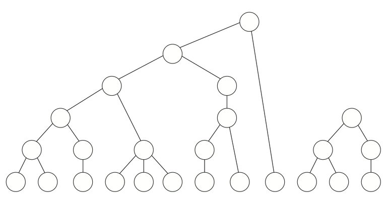
This is an example of such a forest. Here I must make a note about drawings in this blog. It's almost impossible for me to draw forests that would actually be generated by union-find, because they will be incredibly shallow. For example, the union-by-rank rule would never make the root of the bigger tree that vertex. Nevertheless, some visual intuition is needed, so I will add such somewhat incorrect figures. I think they are still useful for illustrative purposes.
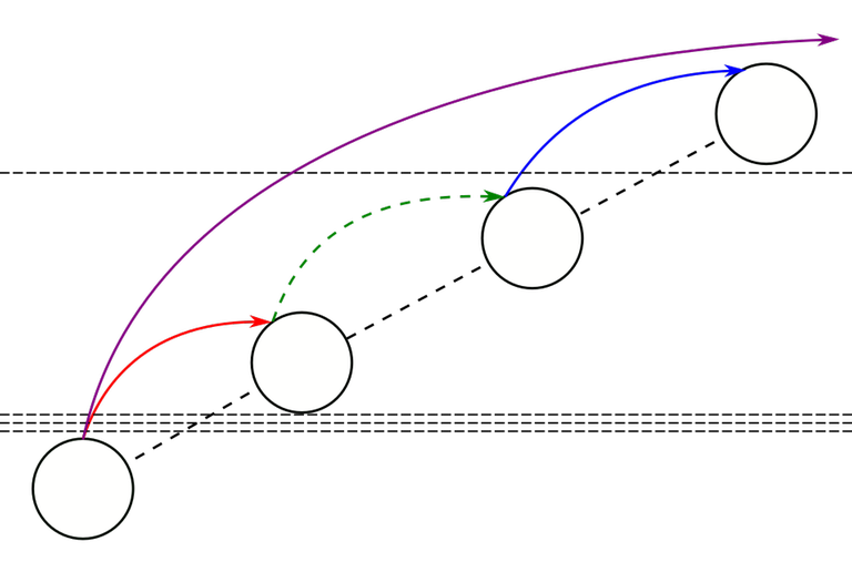
Find-paths and find-edges. Imagine what vertices are visited in some "find" query. If we call find(u), we will visit some ancestors of $$$u$$$, but we might skip some vertices (because these paths have already been compressed). Also, we might stop before the root of the tree because these trees were not joined when the query is made. We will call any path that was created during the course of the algorithm a find-path. Any pair of vertices that are adjacent in a find-path will be called a find-edge.
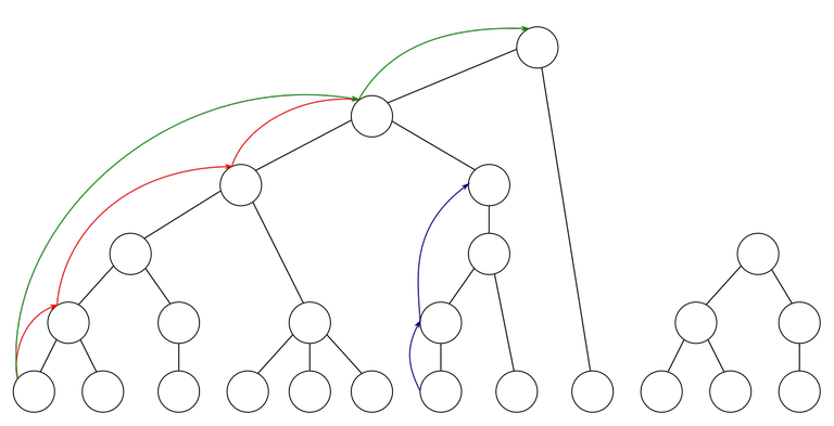
For example, on this figure, some possible find-paths are shown. Each of them shows the path visited during some find query. Notice that, for example, the red find-path jumps over some vertices, because during the actual run of the union-find algorithm, those edges were already compressed by that point. Similarly, it stops before the root, because the root of the forest was not yet in that component when the query was made.
Notice that by the path compression rule, the next find call from $$$u$$$ will generate a find-path that jumps over this entire find-path. An example of this in the image above is the green find-path jumping over the entire red find-path, because after the red query was made, all of that was compressed.
Checklines. Draw the forest in such a way that vertices of the same rank are drawn at the same height. We repeat the following process $$$z$$$ times for some $$$z$$$. For every $$$i$$$ in $$$0 \le i < z$$$:
- Choose some positions $$$0 = a_{i, 0} < a_{i, 1} < a_{i, 2} < a_{i, 3} < \cdots$$$. For every $$$j$$$, we draw a line, called a checkline, of weight $$$i$$$ between the vertices of rank $$$a_{i, j} - 1$$$ and $$$a_{i, j}$$$.
Technically, we draw an infinite number of checklines of weight $$$i$$$, but of course, since the forest has a finite size, there will only be a finite number of checklines that actually matter. Again, right now $$$a_{i, j}$$$ are chosen arbitrarily with relatively few restrictions. During the course of this blog, we will discuss various ways to pick $$$z$$$ and $$$a_{i, j}$$$, and the consequences of these choices. Because you know the end result, you probably know what the best $$$a_{i, j}$$$ end up being but I'm doing it this way to show where these numbers come from.
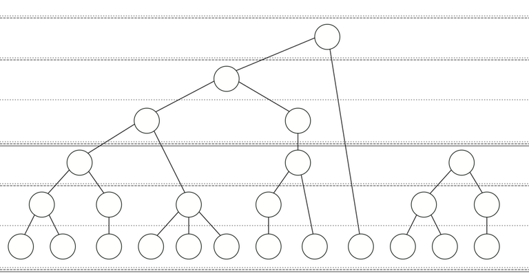
This is a possible example of checkline distribution. Here, we have 3 weights, signified by the dotted, dashed and solid horizontal lines.
"Checkline" is my name for them. Tarjan works directly by comparing ranks with you-know-what, but I find that imagining them as horizontal lines going through the forest emphasizes the intuition of the proof.
Weight of a find-edge. The weight of a find-edge is the smallest $$$k$$$ such that the find-edge passes over no checklines of weight $$$k$$$. For example:
- A find-edge that passes over no checklines has weight 0.
- A find-edge that passes over some checklines of weight 0, but none of weight 1, has weight 1.
- A find-edge that passes over some checklines of weight 0 and 1, but none of weight 2, has weight 2.
- A find-edge that passes over a checkline of every weight has weight $$$z$$$.
Terminality. The proof that we're about to see treats find-edges differently if it is the last (topmost) edge of its weight in its find-path. This is related to the fact that the overall last edge in the find-path is the only one whose parent doesn't change after the find operation. I got tired of writing "find-edge with weight $$$i$$$ such that it is not the last find-edge with weight $$$i$$$ in its path", thus I decided to give it a name.
- A find-edge with weight $$$k$$$ is called $$$k$$$-terminal, if it is the last (topmost) edge of its weight in its find-path.
- A find-edge with weight $$$k$$$ is called $$$k$$$-nonterminal, if it is not $$$k$$$-terminal.
Every find-edge is either $$$k$$$-terminal or $$$k$$$-nonterminal for some $$$k$$$.
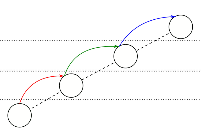
On this figure, there are 2 weights of checklines: dotted (weight 0) and dashed (weight 1). The red, green and blue find-edges here comprise a find-path.
The weights of the edges are:
- The red edge has weight 1 because it passes over a weight-0 checkline but no weight-1 checkline.
- The green edge has weight 2 because it passes over both a weight-0 and a weight-1 checkline.
- The blue edge also has weight 1 similarly to the red edge.
From there we can see which edges are terminal:
- The red edge is 1-nonterminal (because the blue edge also has weight 1 and is further along the path).
- The green edge is 2-terminal because there is no edge with weight 2 further along.
- The blue edge is 1-terminal because there is no edge with weight 1 further along.
Bounding the number of find-edges
The complexity of the algorithm hinges on the number of find-edges, because that is the number of calls to find in the algorithm (including the recursive calls). Every other operation takes constant time, either per query or per find call. We also have the initialization, which takes $$$\mathcal{O}(n)$$$ time, but in all cases we discuss, the number of find-edges in the worst case depends at least linearly on the number of vertices, so initialization is never the bottleneck. Thus, to give an upper bound on the complexity of the algorithm, we calculate an upper bound on the number of find-edges.
I introduced the ideas of terminality and nonterminality for a reason: they behave quite differently. If I have a terminal find-edge, it may also appear in a future find-path. A nonterminal find-edge will not appear again, the next find-edge from that vertex will be "much longer". Therefore, it makes sense to count terminal and nonterminal find-edges separately. Terminal find-edges are easy to deal with:
Observation 3. For any $$$i$$$, the number of $$$i$$$-terminal find-edges is $$$\mathcal{O}(m)$$$.
The number of terminal find-edges will always be $$$\mathcal{O}(zm)$$$. The rest of this blog will be dedicated to counting the number of nonterminal find-edges.
The critical observation and the reason to introduce checklines is the following.
Observation 4. Let $$$i$$$ satisfy $$$1 \le i \le z$$$ and $$$v \to w$$$ be a $$$i$$$-nonterminal find-edge. Suppose $$$v \to w$$$ passes over $$$k$$$ checklines of weight $$$i - 1$$$. If a subsequent find-path contains an edge of the form $$$v \to u$$$, then $$$v \to u$$$ will pass over at least $$$k + 1$$$ checklines of weight $$$i - 1$$$.
The proof of this is so important I won't put it under a spoiler.
Proof. By the definition of $$$i$$$-nonterminality the find-path containing $$$v \to w$$$ looks like $$$\cdots \to v \to w \to \cdots \to v' \to w' \to \cdots \to r$$$, where $$$v' \to w'$$$ is another find-edge with weight $$$i$$$. By the definition of weight, $$$v' \to w'$$$ passes over a checkline of weight $$$i - 1$$$. Because of the path compression rule, after this query, the parent of $$$v$$$ is set to $$$r$$$, which means that any subsequent find-edge from $$$v$$$ must be of the form $$$v \to u$$$, where $$$u$$$ is some ancestor of $$$r$$$. This passes over all $$$k$$$ checklines $$$v \to w$$$ passes over, and also passes over the checkline that $$$v' \to w'$$$ passes over. □
This image hopefully gives some intuition about this. Again, the red, blue and green edge comprise one find-path. Here, we have only one weight of checklines. The red edge is 1-nonterminal and passes over 3 checklines. The blue edge also has weight 1 and thus must pass over a checkline. The next time a find-edge starts from the bottom-left vertex, it must, by path compression, pass over both the red and blue find-edges completely. In this figure, this next find-edge is the purple edge, and it is easy to see that it passes over all 4 checklines in question.
We will use checklines as a way to bound the number of nonterminal edges a vertex $$$v$$$ appears on, because find-edges starting with $$$v$$$ pass over increasingly more checklines. By strategically placing checklines of various weights you can say things like "$$$v$$$ is the lower endpoint in at most $$$x$$$ $$$i$$$-nonterminal find-edges, because it passes over one more checkline of weight $$$i - 1$$$ every time, and after that it must pass over a checkline of weight $$$i$$$.".
Let's do some simple examples of this type of reasoning before we move on to the big guns.
Square-root bound
Denote $$$h$$$ as the height of the forest. There will be two weights of checklines:
- $$$a_{0, j} = j$$$ for every $$$j$$$;
- $$$a_{1, j} = j \lfloor \sqrt{h} \rfloor$$$ for every $$$j$$$.
That is: there is a checkline of weight 0 between every rank, and once every approximately $$$\sqrt{h}$$$ ranks, there is a checkline of weight 1.
For any vertex $$$v$$$, the number of 1-nonterminal find-edges starting at $$$v$$$ is at most $$$\sqrt{h}$$$: every 1-nonterminal find-edge starting at $$$v$$$ will pass over at least one more weight-0 checkline than the last, and after $$$\sqrt{h}$$$ checklines, we are bound to hit a checkline of weight 1.
Similarly, the number of 2-nonterminal find-edges starting at $$$v$$$ is at most $$$\sqrt{h}$$$: every 2-nonterminal find-edge starting at $$$v$$$ will pass over at least one more weight-1 checkline than the last, and after $$$\sqrt{h}$$$ such checklines we pass the highest rank in the forest.
To sum up:
- There are $$$\mathcal{O}(m)$$$ terminal find-edges.
- There are $$$\mathcal{O}(n \sqrt{h})$$$ 1-nonterminal find-edges.
- There are $$$\mathcal{O}(n \sqrt{h})$$$ 2-nonterminal find-edges.
The number of find-edges is therefore $$$\mathcal{O}(m + n \sqrt{h})$$$. If we use union-by-rank, we get $$$\mathcal{O}(m + n \sqrt{\log n})$$$ complexity, and if we don't, we get $$$\mathcal{O}(m + n \sqrt{n})$$$ complexity.
But we can do better!
Logarithmic bound
Here's another example that's very natural for a competitive programmer to try.
We set $$$a_{i, j} = 2^i j$$$. That is:
- there is a checkline of weight 0 between every rank;
- there is a checkline of weight 1 between every 2 ranks;
- there is a checkline of weight 2 between every 4 ranks;
- there is a checkline of weight 3 between every 8 ranks;
- etc.
In other words, at every other checkline of weight $$$i$$$, there is also a checkline of weight $$$i + 1$$$. There is no reason to have more than $$$\log h$$$ different weights for the checklines.
For any vertex $$$v$$$, and for any weight $$$i$$$, the number of $$$i$$$-nonterminal find-edges starting at $$$v$$$ is at most 1. Every $$$i$$$-nonterminal find-edge will pass over at least one more checkline with weight $$$i-1$$$ than the last, and after that we already run into a checkline with weight $$$i$$$.
Therefore:
- There are $$$\mathcal{O}(m \log h)$$$ terminal find-edges ($$$\mathcal{O}(m)$$$ for every weight).
- There are $$$\mathcal{O}(n)$$$ $$$i$$$-nonterminal find-edges for every $$$i$$$; in total $$$\mathcal{O}(n \log h)$$$ nonterminal find-edges.
The total number of find-edges is $$$\mathcal{O}((n + m) \log h)$$$. If we use union-by-rank, we get $$$\mathcal{O}((n + m) \log \log n)$$$ complexity, and if we don't, we get $$$\mathcal{O}((n + m) \log n)$$$ complexity.
But we can do better!
$$$\log^*$$$ bound
The complexities we derived above are pretty awful, because the distribution of checklines fails to properly account for union-by-rank. Yes, we did use the fact that the height of the forest is at most $$$\log n$$$, but we didn't account for the fact that there are exponentially more vertices at the lower ranks than there are at the higher ranks. Who cares if the handful of vertices at rank 1000 have a lot of find-edges (for some weight) starting at them? If there are a handful of vertices at rank 1000, there must be around $$$2^{1000}$$$ vertices at rank 0! Even if there are many find-edges starting around rank 1000, their number will be negligible compared to the number of find-edges that might start at the low-ranking vertices. For any given weight $$$i$$$, the checklines $$$a_{i, j}$$$ should become increasingly sparse as $$$j$$$ increases.
This next bound will account for that, and as you will see, this observation is immensely powerful. Once again, there will be two weights of checklines.
- $$$a_{0, j} = j$$$ for every $$$j$$$;
- $$$a_{1, j} = \underbrace{2^{2^{\vdots^{2}}}}_{j \text{ times}}$$$ for $$$j > 0$$$ and $$$a_{1, 0} = 0$$$.
Here I have to introduce the notation $$$\log^* n$$$. The expression $$$\log^* n$$$ denotes the number of times you have to take the logarithm to get to 1 or below. The function $$$\log^*$$$ is called iterated logarithm and is sort of an inverse function to this power-tower operation: it's easy to see that there are about $$$\log^* n$$$ checklines of weight 1 before we go above the height of the forest.
As mentioned above, there are exponentially more vertices at the lower ranks than there are at the higher ranks. To make the analysis precise, we need the following result.
Observation 5. Denote $$$S_{i, j}$$$ as the number of vertices that are between the $$$j$$$-th and $$$j+1$$$-st checklines of weight $$$i$$$. Then $$$S_{i, j} \le \cfrac{2n}{2^{a_{i, j}}}$$$.
Consider a vertex $$$v$$$ between the $$$j$$$-th and $$$j+1$$$-st checklines of weight 1. What is the number of 1-nonterminal find-edges starting at $$$v$$$? Every 1-nonterminal find-edge starting at $$$v$$$ passes over one more checkline of weight 0. At the very worst case, $$$v$$$ is right above the $$$j$$$-th checkline, so there can be at most $$$a_{1, j+1} - a_{1, j}$$$ 1-nonterminal edges starting at $$$v$$$, and after that we will finally pass over a checkline of weight 1. The total number of 1-nonterminal find-edges that originate from somewhere between the $$$j$$$-th and $$$j+1$$$-st checklines is then at most
because $$$a_{1, j + 1} = 2^{a_{1, j}}$$$.
For any $$$v$$$, number of 2-nonterminal find-edges starting at $$$v$$$ is at most $$$\log^* n$$$, because every time we pass over one more checkline with weight 1, and there are only $$$\log^* n$$$ checklines of weight 1 before we go over the height of the forest.
Therefore:
- There are $$$\mathcal{O}(m)$$$ terminal find-edges.
- There are $$$\mathcal{O}(n \log^* n)$$$ 1-nonterminal find-edges.
- There are $$$\mathcal{O}(n \log^* n)$$$ 2-nonterminal find-edges.
The total number of find-edges, and also complexity, is $$$\mathcal{O}(m + n \log^* n)$$$.
But we can do better!
The best bound
Now you hopefully have some understanding about how the distribution of checklines affects the upper bound on the number of find-edges and therefore complexity. At this point I want to remind you that the algorithm never changes. The algorithm works the same way, regardless of the way you decide to analyze it. The actual number of find-edges remains the same no matter what. The only thing that's changing is our ability to estimate the amount. And we must refine the upper bounds by picking better locations for the checklines until we can't anymore.
Now let's push this technique to the limit.
When comparing the square-root bound and logarithmic bound it's kinda clear that allowing more than two weights for checklines is better. And it's not entirely clear but from the analysis it seems that it is hard to improve on the iterated-logarithmic bound without introducing more weights: the distribution "seems optimal" with respect to the proof technique.
This time around, I'll try to first generalize the proof strategy of the iterated logarithm bound to work with multiple weights, and then pick the distribution of the checklines. Fix $$$i$$$ with $$$0 < i < z$$$ (I remind you that $$$z$$$ was the number of weights: $$$z-1$$$ is the highest weight for a checkline). Suppose that we somehow proved that the number of $$$i$$$-nonterminal find-edges starting at some vertex between the $$$j$$$-th and $$$j+1$$$-th checkline of weight $$$i$$$ is $$$x_{i, j}$$$. Then, the number of $$$i$$$-nonterminal find-edges is
I declare that I want this value to be $$$\mathcal{O}(n)$$$, or alternatively, I want the series
to converge to a value that doesn't depend on $$$n$$$ or $$$i$$$. Why? Because then, the number of nonterminal find-edges will be $$$\mathcal{O}(zn)$$$.
So, we want to decide the values $$$x_{i, j}$$$ such that the series (1) converges. The values $$$x_{i, j}$$$ should be as large as possible, because that means the checklines get as sparse as possible as $$$i$$$ increases, therefore we will more quickly reach the point where there is no reason to add more weights, thus we get to pick a smaller $$$z$$$.
The best way to do this is to let $$$x_{i, j} = a_{i, j}$$$. Then
Note that we could use $$$x_{i, j} = 2 a_{i, j}$$$ or even $$$x_{i, j} = a_{i, j}^{1000}$$$ and get slightly bigger $$$x_{i, j}$$$, but you will see that we are working at the scale of power towers whose heights are determined by other power towers, and such small improvements end up not mattering, at all.
We therefore set out to find a distribution of checklines such that the number of $$$i$$$-nonterminal find-edges starting at some vertex between the $$$j$$$-th and $$$j+1$$$-th checkline of weight $$$i$$$ is $$$a_{i, j}$$$. Let $$$i > 0$$$ and suppose $$$v$$$ is a vertex between the $$$j$$$-th and $$$j+1$$$-th checkline of weight $$$i$$$. The number of $$$i$$$-nonterminal find-edges starting at $$$v$$$ is at most the number of checklines with weight $$$i - 1$$$ that are between the $$$j$$$-th and $$$j+1$$$-th checkline of weight $$$i$$$. So, a nice way to make sure that there are no more than $$$a_{i, j}$$$ such checklines is to set $$$a_{i, j + 1} = a_{i - 1, a_{i, j}}$$$.
Note: we can't have the restriction $$$a_{i, j + 1} = a_{i - 1, a_{i, j}}$$$ if $$$j = 0$$$ because we want $$$a_{i, 0} = 0$$$ to always hold and if we introduce this restriction, then $$$a_{i, j}$$$ will just be 0. We get around this problem by saying that $$$a_{i, j + 1} = a_{i - 1, a_{i, j}}$$$ when $$$i \ge 1, j \ge 1$$$ and that $$$a_{i, 1} = 2$$$ for any $$$i$$$. Then there can be no weight-$$$i$$$ find-edges $$$v \to u$$$ under $$$a_{i, 0} \le \mathrm{rank}(v) < a_{i, 1}$$$ anyway, so this doesn't break our proof.
We have proven the following result.
Observation 6. Let $$$i$$$ satisfy $$$1 \le i < z$$$. If we put certain restrictions on the positions of the checklines $$$a_{i, j}$$$, then the number $$$i$$$-nonterminal find-edges is $$$\mathcal{O}(n)$$$.
The Ackermann function
We have now declared several restrictions on the position $$$a_{i, j}$$$ of the $$$j$$$-th checkline of weight $$$i$$$:
- $$$a_{i, j} < a_{i, j + 1}$$$: just by the definition of what a checkline is;
- $$$a_{i, j} = a_{i - 1, a_{i, j - 1}}$$$ for $$$i \ge 1$$$, $$$j \ge 2$$$: as mentioned, this is the fastest growth rate that lets the series (1) converge;
- $$$a_{i, 0} = 0$$$, $$$a_{i, 1} = 2$$$ for any $$$i$$$: just a base case that makes details work out nicely.
We can complete the last two restrictions into a recursive function by adding a base case for $$$i = 0$$$.
The Ackermann function is the function $$$A \colon\, \mathbb{N} \times \mathbb{N} \to \mathbb{N}$$$ defined by
The function is surely well-defined: if we order all pairs of natural numbers $$$(i, j)$$$ lexicographically, then $$$A(i, j)$$$ will only depend on the values of the pairs before it. This is not the only Ackermann function; many authors define their own version with slightly different base cases, but they all behave very similarly.
This recursive formula really doesn't do the Ackermann function justice, because at least to me it is not immediately obvious that it grows so fast. Many people see the Ackermann function and think that it is just some weird, convoluted function that just happens to grow very fast. But actually, the Ackermann function is something very natural that people often invent when trying to create big numbers. Consider this sequence of the so-called hyperoperations (natural numbers only):
- Multiplication is repeated addition: $$$ab = \underbrace{a + a + \cdots + a}_{b \text{ times}}$$$.
- Exponentiation is repeated multiplication: $$$a^b = a \uparrow b = \underbrace{a \cdot a \cdot \cdots \cdot a}_{b \text{ times}}$$$. The notation $$$a \uparrow b$$$ is Knuth's up-arrow notation; you'll see why it is useful soon.
- Tetration is repeated exponentiation: $$$a \uparrow \uparrow b = \underbrace{a \uparrow (a \uparrow (\cdots (a \uparrow a)))}_{b \text{ times}} = \underbrace{a^{a^{\vdots^{a}}}}_{b \text{ times}}$$$. I have to introduce brackets now because exponentiation is not associative and order of the operations matters.
- Pentation is repeated tetration: $$$a \uparrow \uparrow \uparrow b = \underbrace{a \uparrow\uparrow (a \uparrow\uparrow (\cdots (a \uparrow\uparrow a)))}_{b \text{ times}}$$$
- In general, if we define $$$\uparrow^n$$$ as $$$\underbrace{\uparrow \cdots \uparrow \uparrow}_{n \text{ times}}$$$, then we have $$$a \uparrow^n b = \underbrace{a \uparrow^{n - 1} (a \uparrow^{n - 1} (\cdots (a \uparrow^{n - 1} a)))}_{b \text{ times}}$$$.
The formula for $$$a \uparrow^n b$$$ can alternatively be written as $$$a \uparrow^n b = a \uparrow^{n - 1} (a \uparrow^n (b - 1))$$$. This formula looks very similar to the general case in the Ackermann function: $$$n$$$ plays the role of the first argument, $$$b$$$ plays the role of the second argument and $$$a$$$ is absent in the Ackermann function. So, the hyperoperations follow a similar formula to the Ackermann function. And indeed, using a simple induction we can find out that actually,
So this is what the Ackermann function really is. The first argument tells what kind of hyperoperation — multiplication, exponentiation, tetration, ... — we should use, and the second argument tells us the "exponent". The "base" is always 2. Other versions of the Ackermann function exist and they will have slightly different formulas, but the idea of the formula stays the same. $$$A(i, -)$$$ will have a similar growth rate to the $$$i$$$-th hyperoperation, or perhaps $$$i-1$$$-st or $$$i+1$$$-st hyperoperation, it doesn't really matter.
We introduced the Ackermann function to use it as the locations of the checklines. We want to set $$$a_{i, j} = A(i, j)$$$, but first we should make sure that $$$A(i, j) < A(i, j + 1)$$$ really holds. We can check this by induction on $$$i$$$: for $$$i = 0$$$, the sequence is obviously increasing in $$$j$$$. Now, suppose that and $$$A(i - 1, j) < A(i - 1, j + 1)$$$ for any $$$j$$$. Since $$$A(i - 1, 1) = 2$$$, we have $$$A(i - 1, j) > j$$$ for $$$j > 0$$$. For $$$j > 0$$$ we have $$$A(i, j + 1) = A(i - 1, A(i, j)) > A(i, j)$$$ and $$$A(i, 1) > A(i, 0)$$$ follows from the definition.
Wrapping up the proof
Set $$$a_{i, j} = A(i, j)$$$. It's now time to count the number of 0-nonterminal and $$$z$$$-nonterminal edges.
Observation 7. Using the distribution of checklines given by the Ackermann function, the number of $$$0$$$-nonterminal find-edges is $$$\mathcal{O}(n)$$$.
For any $$$i$$$, $$$A(i, 0) = 0$$$, $$$A(i, 1) = 2$$$ and $$$A(i, 2) = 4$$$. The value of $$$A(i, 3)$$$ grows very rapidly as $$$i$$$ increases. Define the inverse Ackermann function $$$\alpha(n)$$$ as the smallest $$$k$$$ such that $$$A(k, 3) \ge n$$$. Again, this definition differs a bit from the various definitions given in the literature, but ultimately it does not matter very much.
As an aside, there has been some confusion regarding the growth rates of the functions $$$\log^*$$$ and $$$\alpha$$$. While I of course understand that both functions are in practice constants valued 3, in theory $$$\alpha$$$ is an entirely different kind of beast. So if you're interested in the theory, you shouldn't settle for $$$\log^*$$$. I'll let you judge based on this comparison:
while
and $$$\alpha(2 \uparrow^5 3) = 5$$$ yet $$$\log^*(2 \uparrow^5 3)$$$ is already some disgusting number that I can't write down without up-arrows.
If we let $$$z = \alpha(n) + 1$$$, then there will be only $$$\mathcal{O}(1)$$$ checklines of weight $$$z - 1$$$ such that there are vertices above them. Thus, for any vertex $$$v$$$, the number of $$$z$$$-nonterminal find-edges will be $$$\mathcal{O}(1)$$$. We get that the number of $$$z$$$-nonterminal find-edges is $$$\mathcal{O}(n)$$$.
Theorem. The complexity of union-find with path compression and union-by-rank is $$$\mathcal{O}((n + m) \alpha(n))$$$.
Proof. All that's left to do is to sum up the bounds we calculated.
- The number of terminal find-edges is $$$\mathcal{O}(zm)$$$.
- The number of 0-nonterminal find-edges is $$$\mathcal{O}(n)$$$.
- The number of $$$i$$$-nonterminal find-edges for each $$$0 < i < z$$$ is $$$\mathcal{O}(n)$$$.
- The number of $$$z$$$-nonterminal find-edges is $$$\mathcal{O}(n)$$$.
The number of terminal find-edges is $$$\mathcal{O}(zm)$$$ and the number of nonterminal find-edges is $$$\mathcal{O}(zn)$$$, so the total number of find-edges comes to $$$\mathcal{O}(z(n + m))$$$. Since $$$z$$$ is $$$\mathcal{O}(\alpha(n))$$$, the number of find-edges and thus the complexity of the algorithm comes to $$$\mathcal{O}((n + m) \alpha(n))$$$. □
But can we do better?
Optimality
After seeing this complexity and proof, one may think that the Ackermann function is just some idiosyncrasy of our chosen method for bounding the number of find-edges. Besides that, throughout the lower bounds we proved, we had some new ideas every time (notably, the observation that there are exponentially more vertices at lower ranks) that made a smaller complexity possible. And it seems that there is no reason to give up: there might be more new ideas that give even better upper bounds on the complexity.
But this is not the case. In the paper I am explaining here, Tarjan also provides a family of graphs where this algorithm must take at least that many steps. Furthermore, this example shows that the inverse Ackermann runtime is "almost certainly" optimal for the union-find problem. "Almost certainly" means that entirely different union-find algorithms might be better, but algorithms similar to ours will have inverse Ackermann complexity in the worst case. Here, "similar to ours" means:
- Maintains a forest, keeping the parent of each vertex.
- Has some kind of rule about which way to unite trees (union by rank, union by size, union by coin flip etc).
- May use some kind of shortcutting for find (path compression, path halving, path splitting etc).
- But does no other clever thing that can't be formulated as an union rule or a form of shortcutting!
I will not prove this here, because it's... quite long and complicated.


You have put some USA truck service instead of Wikipedia link lol.
Damn. I started writing the draft a few weeks ago and used an URL shortener because CF blogs don't like () in links. But it seems that the link either expired or had a collision...
By the by, HTML works too, so
[X](Y)is completely equivalent to<a href="Y">X</a>except that the latter allows parentheses and other weird syntax.Instructions unclear, my algorithm is now exponential
Thank you for this beautiful proof, you write very well, I spent all night reading this.
I found two typos:
In the proof of observation 4: "where u is some ancestor of u" -> "where u is some ancestor of v (or r?)"
In a note before observation 6: "when i≥1,j≥1" -> "when i≥1,j≥2" because after that you say "ai,1 = 2".
Thanks, I have fixed the first mistake. Indeed $$$r$$$ is correct.
The second is not an error, because I am setting a value to $$$a_{i,j+1}$$$, not $$$a_{i,j}$$$.