You can also read this on my blog: https://mzhang2021.github.io/cp-blog/simulating-cost-flow/

Thanks to gabrielwu for proofreading.

This post assumes knowledge of min/max cost flow and a rough understanding of the high-level methods for solving (successive shortest path and cycle canceling). Knowledge of specific algorithms and implementation details are not expected. Also solutions to some problems will use Aliens trick.

The cost flow problem is a well-known problem in literature that a whole slew of competitive programming problems can be formulated as. Unfortunately, competitive programming problems typically have constraints set too high for directly running even the most state of the art cost flow algorithm. However, in certain problems the flow network will have a very specific setup that allows us to figure out greedily the optimal flow (i.e. proving greedy with flow) or "simulate" the flow algorithm faster with data structures. That is what this post will be about.

I will say that I do not claim novelty over these ideas. This idea is (unsurprisingly) well-known in China. This particular post and some of the example problems are taken from this Chinese blog.

I will also describe everything below in terms of min cost flow, max cost is of course analogous. When describing flow network constructions, I will shorthand with $$$(cost, capacity)$$$ for describing edges.

High-level Methods for Cost Flow

Most cost flow algorithms fall into one of these categories of high-level approaches. The two in particular that we will look at are:

1. Successive Shortest Path: Repeatedly find a min cost augmenting path (a path with minimum total cost where all edges can still contain more flow) from source to sink and send flow through that path.
2. Cycle Cancelling: Repeatedly find a negative cost cycle (a cycle with negative total cost where all edges can still contain more flow) and send flow through that cycle.

Note that in the cycle cancelling paradigm, there is no concept of source and sink, but you can solve for source and sink by adding an edge from sink to source with cost of $$$-\infty$$$ and capacity of $$$k$$$ for the min cost $$$k$$$-flow (or $$$\infty$$$ capacity if you want min cost max flow).

Min Cost Flow is Convex

Min cost flow as a function of amount of flow is convex. This makes intuitive sense, as you can always rearrange the augmenting paths you choose to pick less steep ones (lower cost) before more steep ones (higher cost). This fact is useful as it allows us to use Aliens trick.

Codeforces 802O: April Fools' Problem

Statement Summary: You are preparing and printing $$$k$$$ problems for a contest over the course of $$$n$$$ days. On the $$$i$$$th day, you can prepare a problem for cost $$$a_i$$$ and print a problem for cost $$$b_i$$$. You must prepare a problem before printing it. In other words, if you prepare a problem on day $$$i$$$, you can only print it on some day $$$j \geq i$$$. You can prepare and print at most one problem per day. What is the minimum cost of preparing and printing $$$k$$$ problems?

Constraints: $$$1 \leq k \leq n \leq 5 \cdot 10^5, 1 \leq a_i, b_i \leq 10^9$$$

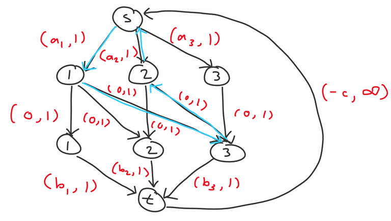
Let's first think about solving this with flows. One straightforward way is to create $$$2n + 2$$$ nodes: a source $$$s$$$ and sink $$$t$$$, plus nodes representing $$$a_i$$$ and $$$b_i$$$ for each $$$i$$$. We add the following edges:

• $$$s$$$ to each $$$a_i$$$ node with $$$(a_i, 1)$$$
• each $$$b_i$$$ node to $$$t$$$ with $$$(b_i, 1)$$$
• each $$$a_i$$$ node to $$$b_j$$$ node where $$$i \leq j$$$ with $$$(0, 1)$$$

The answer is the min cost $$$k$$$-flow of this network.

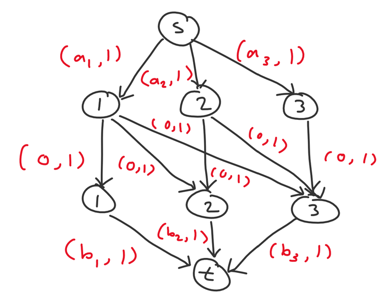
Example for $$$n = 3$$$

Now let's try to optimize using one of two methods. Both are possible and lead to different solutions for this problem.

Successive Shortest Path

This is the method described in the official editorial.

First, let's simplify this network to not use $$$\Omega(n^2)$$$ edges. Consider a slightly different setup with $$$n + 2$$$ nodes: a source $$$s$$$ and sink $$$t$$$, plus nodes $$$1$$$ through $$$n$$$. We add the following edges:

• $$$s$$$ to each $$$i$$$ with $$$(a_i, 1)$$$
• each $$$i$$$ to $$$t$$$ with $$$(b_i, 1)$$$
• $$$i$$$ to $$$i + 1$$$ with $$$(0, \infty)$$$

I claim the answer is also the min cost $$$k$$$-flow of this network. Essentially, a matching consists of picking some $$$a_i$$$, waiting zero or more days (represent by taking some number of $$$i \to i + 1$$$ edges), and then pick some $$$b_j$$$ where $$$i \leq j$$$.

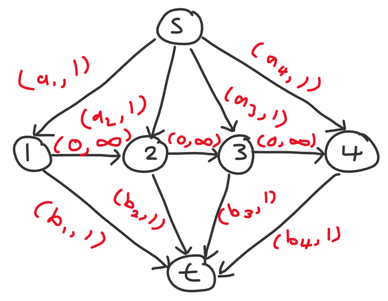
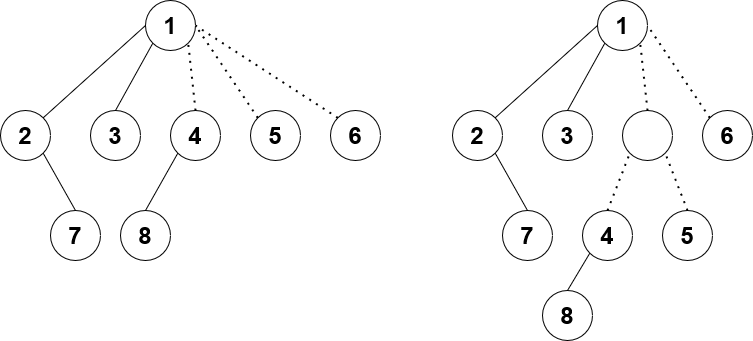
Example for $$$n = 4$$$

An augmenting path consists of sending flow from $$$s$$$ to some $$$i$$$, then from $$$i$$$ to $$$j$$$, and finally from $$$j$$$ to $$$t$$$.

• $$$s \to i$$$ and $$$j \to t$$$ must of course have no flow going through them.
• If $$$i \leq j$$$, this is ok. We add $$$+1$$$ flow to each edge on the path from $$$i$$$ to $$$j$$$.
• If $$$i > j$$$, then we are sending flow along a reverse edge and cancelling out existing flow, so every edge on the path from $$$i$$$ to $$$j$$$ must have at least $$$1$$$ flow, and the augmenting path adds $$$-1$$$ flow to each path edge.

And in the successive shortest path algorithm, we simply need to choose the augmenting path with minimum cost each time. So we need to choose a pair of indices $$$i, j$$$ with minimum $$$a_i + b_j$$$, and either $$$i \leq j$$$ or there exists flow on every edge on the path between $$$i$$$ and $$$j$$$.

So we need to be able to add $$$+1$$$ or $$$-1$$$ to a range and recompute the minimum cost valid $$$(i, j)$$$ pair. This sounds like a job for lazy segment tree! We just repeat $$$k$$$ times of querying the segtree for $$$(i, j)$$$ and either add $$$+1$$$ or $$$-1$$$ to all edges in between $$$i$$$ and $$$j$$$, giving us an $$$\mathcal O(k \log n)$$$ solution.

The details for determining the minimum cost valid $$$(i, j)$$$ pair are quite tedious, but the TLDR is that you have to store first and second minimums of the amount of flow through any edge in a subarray. I have an old submission that implements this idea with a ton of variables in the segtree node. It can probably be reduced with more thought.

Cycle Cancelling

To drastically simplify our analysis, we will apply Aliens trick. Binary search on some reward $$$c$$$, so now there is no requirement of at least $$$k$$$ problems anymore, but instead you get a reward of $$$c$$$ for completing one problem. So preparing a problem on day $$$i$$$ and printing on day $$$j$$$ costs $$$a_i + b_j - c$$$. So there is an edge from $$$t$$$ to $$$s$$$ with $$$(-c, \infty)$$$. We binary search for the minimum $$$c$$$ that we complete at least $$$k$$$ problems. This is valid because we know min cost flow is convex with respect to the amount of flow.

Now consider incrementally adding in nodes in decreasing order (from $$$n$$$ to $$$1$$$) and consider how the optimal flow changes after each additional node. When we add node $$$i$$$, we add edges $$$s \to a_i$$$, $$$b_i \to t$$$, and $$$a_i \to b_j$$$ for all $$$i \leq j$$$. Upon adding node $$$i$$$, we consider the possibilities for how a new negative cycle could form.

1. $$$s \to a_i \to b_j \to t \to s$$$ with cost $$$a_i + b_j - c$$$. This is essentially matching $$$a_i$$$ with some unmatched $$$b_j$$$.
2. $$$s \to a_i \to b_j \to a_k \to s$$$ with cost $$$a_i - a_k$$$. This is cancelling out some existing flow passing through $$$s \to a_k \to b_j$$$ and is equivalent to changing the matching to match $$$b_j$$$ with $$$a_i$$$ instead of $$$a_k$$$.

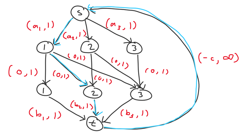
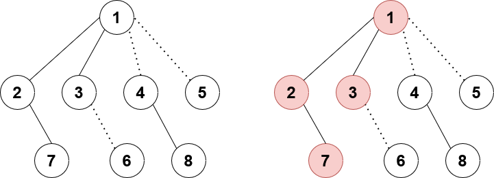
Examples of negative cycles of the first and second types

Those are actually the only two cases we need to consider. For example, you might think we need to consider some cycle of the form $$$s \to a_i \to b_j \to t \to b_k \to a_l \to s$$$. This cycle would represent taking some matched pair $$$(a_i, b_j)$$$ instead of $$$(a_l, b_k)$$$. However, if $$$(a_l, b_k)$$$ was originally matched in the first place, that would imply $$$a_l + b_k \leq c$$$, as otherwise $$$t \to b_j \to a_i \to s \to t$$$ would be a negative cycle with weight $$$c - a_l - b_k$$$ and we would have had to handle that before adding node $$$i$$$. And if $$$s \to a_i \to b_j \to t \to b_k \to a_l \to s$$$ was a negative cycle, that would imply $$$a_i + b_j < a_l + b_k$$$ and therefore $$$a_i + b_j < c$$$, so we could instead take the negative cycle $$$s \to a_i \to b_j \to t \to s$$$. In fact, we would ultimately converge to that state regardless, because if we took $$$s \to a_i \to b_j \to t \to b_k \to a_l \to s$$$ first, then $$$s \to a_l \to b_k \to t \to s$$$ would form a negative cycle afterwards, so the end result after resolving all negative cycles is identical.

You can also confirm that after taking a negative cycle of one of the two types listed above (whichever one is more negative), we will not create any more additional negative cycles. So essentially, each time we add a node $$$i$$$ to the network, we take at most one additional negative cycle.

Therefore, we can simply maintain a priority queue of potential negative cycles and iterate $$$i$$$ from $$$n$$$ to $$$1$$$. When we match $$$(a_i, b_j)$$$, we insert $$$-a_i$$$ into the priority queue to allow for breaking up that matching and pairing $$$b_j$$$ with something else in the future. When we leave $$$b_i$$$ unmatched, we insert $$$b_i - c$$$ into the priority queue to allow for matching with that $$$b_i$$$ in the future. And at each step, if $$$a_i$$$ plus the minimum value in the priority queue is less than $$$0$$$, then we take that option. The overall complexity is $$$\mathcal O(n \log n \log A)$$$ (but with much better constant than the successive shortest path solution).

auto solve = [&] (int c) -> pair<int, long long> {
    int cnt = 0;
    long long cost = 0;
    priority_queue<pair<int, int>, vector<pair<int, int>>, greater<pair<int, int>>> pq;
    for (int i=n-1; i>=0; i--) {
        pq.emplace(b[i] - c, 0);
        if (a[i] + pq.top().first <= 0) {
            cnt += pq.top().second == 0;
            cost += a[i] + pq.top().first;
            pq.pop();
            pq.emplace(-a[i], 1);
        }
    }
    return {cnt, cost + (long long) k * c};
};

int l = 0, r = 2e9 + 5;
while (l < r) {
    int m = midpoint(l, r);
    if (solve(m).first >= k)
        r = m;
    else
        l = m + 1;
}

cout << solve(l).second << "\n";

Notice that the final solution looks awfully similar to a greedy algorithm. And indeed, we can apply a greedy interpretation to this: each $$$a_i$$$ can be matched with some $$$b_j$$$ where $$$i \leq j$$$ for cost $$$a_i + b_j - c$$$, and we want cost as negative as possible. Then the two types of negative cycles can be interpreted as "options" when introducing a new index $$$i$$$: either match $$$a_i$$$ with some unmatched $$$b_j$$$ or swap it with some existing $$$(a_k, b_l)$$$ matching. In essence, the flow interpretation serves as a proof for the correctness of the greedy.

5 3
9 1 10 10 4
6 7 8 2 9

So with this first example, we can see two different solutions that arise from thinking about flows. The first one is probably impossible to think of without flows. For the second one, it might be difficult to prove Aliens trick can be applied here without formulating it as flow. Once Aliens trick is applied, the greedy is relatively easier to come up without thinking about flows, but having the flow network still gives us confidence in its correctness.

Codeforces 866D: Buy Low Sell High

Statement Summary: You have knowledge of the price of a stock over the next $$$n$$$ days. On the $$$i$$$th day it will have price $$$p_i$$$. On each day you can either buy one share of the stock, sell one existing share you currently have, or do nothing. You cannot sell shares you do not have. What is the maximum possible profit you can earn?

Constraints: $$$2 \leq n \leq 3 \cdot 10^5, 1 \leq p_i \leq 10^6$$$

This problem has several interpretations that lead to the same code. You can think of it as slope trick. Or as greedy. Let's think about it as flows.

Firstly, we can loosen the restrictions by allowing for both buying and selling a stock on a given day. This won't change the answer since both buying and selling on the same day is equivalent to doing nothing.

Now we design the following flow network with $$$n + 2$$$ nodes: a source $$$s$$$ and sink $$$t$$$ and $$$n$$$ nodes representing days $$$1$$$ through $$$n$$$. We add the following edges:

• $$$s$$$ to $$$i$$$ for all $$$1 \leq i \leq n$$$ with $$$(-p_i, 1)$$$
• $$$i$$$ to $$$t$$$ for all $$$1 \leq i \leq n$$$ with $$$(p_i, 1)$$$
• $$$i$$$ to $$$i + 1$$$ for all $$$1 \leq i < n$$$ with $$$(0, \infty)$$$

The answer is thus the max cost flow of this network.

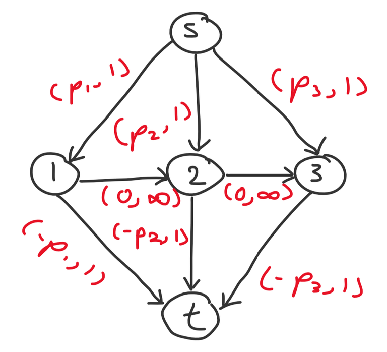
Example for $$$n = 3$$$

Now consider the cycle cancelling method. Add an edge from $$$t$$$ to $$$s$$$ with $$$(0, \infty)$$$. We are using a cost of $$$0$$$ instead of $$$\infty$$$ because we do not require the max amount of flow, and forcing the max flow is not always optimal.

This network is extremely similar to the previous problem. We add the nodes from $$$n$$$ to $$$1$$$. When we add node $$$i$$$, the possible positive (since we are doing max cost flow) cycles are:

• $$$s \to i \to \dots \to j \to t \to s$$$ for $$$i \leq j$$$ with cost $$$p_j - p_i$$$
• $$$s \to i \to \dots \to j \to s$$$ for $$$i \leq j$$$ also with cost $$$p_j - p_i$$$

So the code ends up being quite simple and may resemble some other greedy code you've seen.

long long ret = 0;
priority_queue<int> pq;
for (int i=n-1; i>=0; i--) {
    pq.push(p[i]);
    if (pq.top() > p[i]) {
        ret += pq.top() - p[i];
        pq.pop();
        pq.push(p[i]);
    }
}

CSES Programmers and Artists

Statement Summary: You have $$$n$$$ people, the $$$i$$$th person has $$$x_i$$$ amount of programming skill and $$$y_i$$$ amount of art skill. Each person can be assigned to be a programmer, artist, or neither. You need exactly $$$a$$$ programmers and $$$b$$$ artists. What is the maximum sum of skills attainable by some matching?

Constraints: $$$1 \leq n \leq 2 \cdot 10^5, a + b \leq n, 1 \leq x_i, y_i \leq 10^9$$$

You get the drill now. Let's model this problem as a flow network. Here is one possible construction using $$$n + 4$$$ nodes.

• $$$s$$$ to $$$i$$$ with $$$(0, 1)$$$
• $$$i$$$ to $$$prog$$$ with $$$(x_i, 1)$$$
• $$$i$$$ to $$$art$$$ with $$$(y_i, 1)$$$
• $$$prog$$$ to $$$t$$$ with $$$(0, a)$$$
• $$$art$$$ to $$$t$$$ with $$$(0, b)$$$

The answer is the max cost max flow of this network. Notice that in this case the maximum flow is also optimal as all augmenting paths will have positive weight.

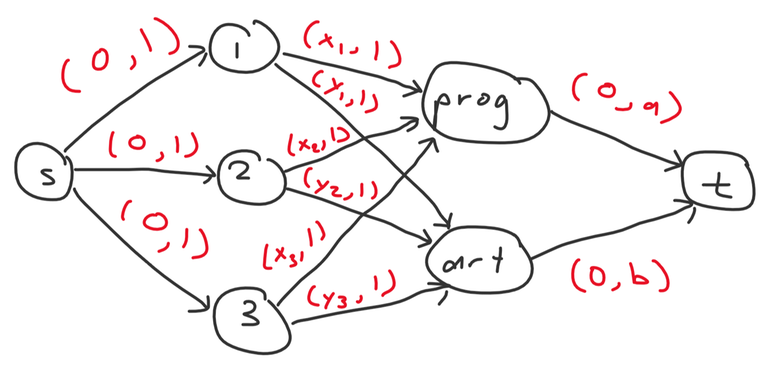
Example for $$$n = 3$$$

Let's try approaching this with successive shortest path! Essentially, we repeatedly find an augmenting path from $$$s$$$ to $$$t$$$ with maximum cost and send $$$1$$$ unit of flow through. After some pondering, we conclude we only have $$$4$$$ types of paths to consider.

• $$$s \to i \to prog \to t$$$ with cost $$$x_i$$$
• $$$s \to i \to art \to t$$$ with cost $$$y_i$$$
• $$$s \to i \to prog \to j \to art \to t$$$ with cost $$$x_i - x_j + y_j$$$
• $$$s \to i \to art \to j \to prog \to t$$$ with cost $$$y_i - y_j + x_j$$$

The first and fourth types of paths decrease the capacity of $$$prog \to t$$$ by $$$1$$$, and the second and third types of paths decrease the capacity of $$$art \to t$$$ by $$$1$$$.

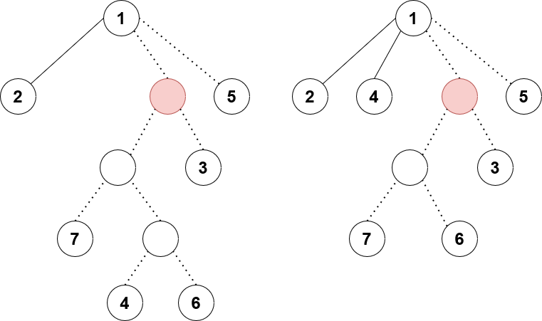
Do we need to consider any more complicated paths? Such as $$$s \to i \to prog \to j \to art \to k \to prog \to t$$$? Turns out we don't. Suppose path $$$s \to i \to prog \to j \to art \to k \to prog \to t$$$ has the maximum cost. The cost is $$$x_i - x_j + y_j - y_k + x_k$$$. Now consider a different augmenting path that would also be valid, $$$s \to i \to prog \to t$$$ with cost $$$x_i$$$. The fact that the other path was chosen implies $$$x_i - x_j + y_j - y_k + x_k > x_i$$$, or $$$y_j - x_j + x_k - y_k > 0$$$. This implies that there exists a positive cycle $$$j \to art \to k \to prog \to j$$$ before introducing our new augmenting path, contradicting the property of successive shortest paths which ensures optimal cost flow with each new augmenting path added.

Therefore, we just need to maintain some heaps to repeatedly find the maximum cost path out of those $$$4$$$ options:

• pair unmatched $$$i$$$ to programmer
• pair unmatched $$$i$$$ to artist
• pair unmatched $$$i$$$ to programmer, and switch some existing programmer $$$j$$$ to artist
• pair unmatched $$$i$$$ to artist, and switch some existing artist $$$j$$$ to programmer

My code is a bit verbose but attempts to implement this idea as straightforwardly as possible:

#include <bits/stdc++.h>
using namespace std;

#ifdef LOCAL
#define DEBUG(...) debug(#__VA_ARGS__, __VA_ARGS__)
#else
#define DEBUG(...) 6
#endif

template<typename T, typename S> ostream& operator << (ostream &os, const pair<T, S> &p) {return os << "(" << p.first << ", " << p.second << ")";}
template<typename C, typename T = decay<decltype(*begin(declval<C>()))>, typename enable_if<!is_same<C, string>::value>::type* = nullptr>
ostream& operator << (ostream &os, const C &c) {bool f = true; os << "["; for (const auto &x : c) {if (!f) os << ", "; f = false; os << x;} return os << "]";}
template<typename T> void debug(string s, T x) {cerr << "\033[1;35m" << s << "\033[0;32m = \033[33m" << x << "\033[0m\n";}
template<typename T, typename... Args> void debug(string s, T x, Args... args) {for (int i=0, b=0; i<(int)s.size(); i++) if (s[i] == '(' || s[i] == '{') b++; else
if (s[i] == ')' || s[i] == '}') b--; else if (s[i] == ',' && b == 0) {cerr << "\033[1;35m" << s.substr(0, i) << "\033[0;32m = \033[33m" << x << "\033[31m | "; debug(s.substr(s.find_first_not_of(' ', i + 1)), args...); break;}}

template<typename T>
struct FastSet {
    priority_queue<T> pq, pending;

    void add(T x) {
        pq.push(x);
    }

    void rem(T x) {
        pending.push(x);
        while (!pq.empty() && !pending.empty() && pq.top() == pending.top()) {
            pq.pop();
            pending.pop();
        }
    }

    T max() {
        assert(!pq.empty());
        return pq.top();
    }
};

int main() {
    ios_base::sync_with_stdio(false);
    cin.tie(NULL);

    int a, b, n;
    cin >> a >> b >> n;
    vector<int> x(n), y(n);
    for (int i=0; i<n; i++)
        cin >> x[i] >> y[i];

    FastSet<pair<int, int>> pqA, pqB;
    priority_queue<pair<int, int>> pqA2, pqB2;
    for (int i=0; i<n; i++) {
        pqA.add({x[i], i});
        pqB.add({y[i], i});
    }

    long long ret = 0;
    while (a > 0 || b > 0) {
        int mx = 0;
        if (a > 0) {
            if (!pqA.pq.empty())
                mx = max(mx, pqA.max().first);
            if (!pqB.pq.empty() && !pqB2.empty())
                mx = max(mx, pqB.max().first + pqB2.top().first);
        }
        if (b > 0) {
            if (!pqB.pq.empty())
                mx = max(mx, pqB.max().first);
            if (!pqA.pq.empty() && !pqA2.empty())
                mx = max(mx, pqA.max().first + pqA2.top().first);
        }
        assert(mx > 0);

        ret += mx;
        if (a > 0) {
            if (!pqA.pq.empty() && mx == pqA.max().first) {
                int i = pqA.max().second;
                pqA.rem({x[i], i});
                pqB.rem({y[i], i});
                pqA2.emplace(y[i] - x[i], i);
                a--;
                continue;
            }
            if (!pqB.pq.empty() && !pqB2.empty() && mx == pqB.max().first + pqB2.top().first) {
                int i = pqB.max().second, j = pqB2.top().second;
                pqA.rem({x[i], i});
                pqB.rem({y[i], i});
                pqB2.pop();
                pqB2.emplace(x[i] - y[i], i);
                pqA2.emplace(y[j] - x[j], j);
                a--;
                continue;
            }
        }
        if (b > 0) {
            if (!pqB.pq.empty() && mx == pqB.max().first) {
                int i = pqB.max().second;
                pqA.rem({x[i], i});
                pqB.rem({y[i], i});
                pqB2.emplace(x[i] - y[i], i);
                b--;
                continue;
            }
            if (!pqA.pq.empty() && !pqA2.empty() && mx == pqA.max().first + pqA2.top().first) {
                int i = pqA.max().second, j = pqA2.top().second;
                pqA.rem({x[i], i});
                pqB.rem({y[i], i});
                pqA2.pop();
                pqA2.emplace(y[i] - x[i], i);
                pqB2.emplace(x[j] - y[j], j);
                b--;
                continue;
            }
        }
        assert(false);
    }

    cout << ret << "\n";

    return 0;
}

More Problems

• Codeforces 280D: k-Maximum Subsequence Sum
• NOI 2019: Sequence
• CCPC Finals 2021 Problem I: Reverse LIS
• Any other example problem from this blog

Hey everyone! Usually when I post stuff on CF I just drop an external link to my blog, but this time I would like to also paste the same content natively on CF to see if it leads to more engagement. You can read the exact same article on my blog here.

Also, special thanks to alien_lover and gabrielwu for proofreading.

Motivation

We will solve this problem.

Prologue

The original name of this problem is SONE1, originating from the fiery depths of Chinese OI. Amazingly, the Chinese have figured out how to augment the link/cut tree to solve this problem (ref 1, 2). Maintaining subtree aggregates with a LCT isn't difficult, and there's a well-known Codeforces article by ouuan about it, but supporting lazy subtree updates is much harder. There's this, but it requires the updates to be invertible. I haven't found any English resources explaining how to augment LCT to solve this problem, so this article is my attempt at doing that. Most of the content is credited to this article, and the implementation is built upon a clean ordinary LCT implementation by bicsi.

EDIT: As an aside, some readers have pointed out that this is essentially what's referred to in English as a "Top Tree". The articles I referenced referred to it as an "AAA Tree". I initially assumed they were different, but after skimming the paper in question there indeed seem to be similarities, just differences in what stuff are called.

Prerequisites

• Link/Cut Tree
  • https://en.wikipedia.org/wiki/Link/cut_tree
  • https://www.youtube.com/watch?v=XZLN6NxEQWo
• Supporting Subtree Aggregates (But Not Lazy) with LCT
  • https://codeforces.com/blog/entry/67637

Terminology

I will use the same terminology used in the resources linked in the prerequisites section. Here is a complete list of them to ensure we are all on the same page before proceeding:

The Core Idea

I have a LCT, and I store the aggregates of each subtree in virtual subtrees. Any child of a node is either a preferred child or a virtual child. The issue with doing lazy propagation directly on this model is that a node could have several (up to $$$\mathcal O(n)$$$) virtual subtrees hanging from it, and we cannot push down the lazy tags to each of its virtual children each time. The fix is surprisingly simple: binarize the tree. This way, when we push down lazy tags, we only have at most two virtual children to push to, and the complexity is fixed. To understand what I mean by binarize, take a look at the diagram of LCTs below:

The solid lines represent preferred edges, and the dotted lines are unpreferred/virtual edges. The nodes 2, 7, 1, 3 form a preferred path in that order. Node 1 has both a left and right preferred child, and it has 3 virtual children.

The LCT on the left is what an ordinary LCT might look like. Node 1 has 3 virtual children, which is more than 2. Therefore, we binarize its virtual children by introducing a new fake vertex to connect both 4 and 5. Now as seen in the LCT on the right, each node has at most 2 preferred children and 2 virtual children (up to 4 children in total). So simple!

If only... the devil is in the details...

If you were to go and start coding this idea right now, you might realize there are quite few pitfalls to keep in mind while coding. The next few sections will be dedicated to talking about some of the implementation details in depth.

The Access Method

Since everything in LCTs revolve around access, let's first characterize the access method. Here's what a typical access method might look like:

// tr is a global array storing each of the LCT nodes
// p is the parent and ch is a size 4 array of its children
void attach(int u, int d, int v) {
    tr[u].ch[d] = v;
    tr[v].p = u;
    pull(u);
}

// adds v as a virtual child of u
void add(int u, int v) {
    tr[u].vir += tr[v].sum;
}

// removes v as a virtual child of u
void rem(int u, int v) {
    tr[u].vir -= tr[v].sum;
}

void access(int u) {
    splay(u);
    add(u, tr[u].ch[1]);        // the preferred path ends at u, so any node with greater depth should be disconnected and made virtual instead
    attach(u, 1, 0);            // sets the right preferred child of u to null (0)
    while (tr[u].p) {
        int v = tr[u].p;
        splay(v);
        add(v, tr[v].ch[1]);    // disconnect any node with greater depth than v, so result is a preferred path ending at v
        rem(v, u);              // u is no longer a virtual child of v
        attach(v, 1, u);        // u is now the right preferred child of v
        splay(u);
    }
}

You'll be glad to hear this isn't far from the final product. The fundamental process of accessing a node remains the same. The only difference is that the add and rem methods become more complex, because we may have to introduce more fake nodes for binarization.

The Add Method

Firstly, let's take a look at add.

// attaches v as a virtual child of u
void add(int u, int v) {
    if (!v)
        return;
    for (int i=2; i<4; i++)
        if (!tr[u].ch[i]) {
            attach(u, i, v);
            return;
        }
    int w = newFakeNode();
    attach(w, 2, tr[u].ch[2]);
    attach(w, 3, v);
    attach(u, 2, w);
}

The first case is straightforward: if one of our 2 virtual children is null, simply set $$$v$$$ as that virtual child instead.

for (int i=2; i<4; i++)
    if (!tr[u].ch[i]) {
        attach(u, i, v);
        return;
    }

The second case is when $$$u$$$ already has 2 virtual children. In that case, we create a new fake node connecting both $$$v$$$ and one of our old virtual children, and substituting that as the new virtual child.

int w = newFakeNode();
attach(w, 2, tr[u].ch[2]);
attach(w, 3, v);
attach(u, 2, w);

The rem method is slightly more complex and requires the introduction of several other concepts first, so we'll come back to that in a minute.

Bound on Fake Node Creation

Firstly, while we're on the subject of fake nodes, how many fake nodes will we create? If we only create fake nodes without destroying, we could create as many as the number of preferred child changes, which is $$$\mathcal O(n \log n)$$$ with significant constant. That's often an undesirable amount of memory to use. Fortunately, observe that at any point, we only need at most $$$n$$$ fake nodes to binarize the entire tree. Therefore, as long as we recycle memory and destroy fake nodes in the rem method when they become unnecessary, we will limit our memory usage to just $$$2n$$$ nodes.

Fake Nodes in Our Preferred Paths?

If we just splay willy-nilly in our access method, we might connect fake nodes into our preferred paths. This is undesirable because it becomes messy to keep track of where fake nodes are and when we can destroy them for preserving memory. Thus, we'll need to make the following change to access.

void access(int u) {
    splay(u);
    add(u, tr[u].ch[1]);
    attach(u, 1, 0);
    while (tr[u].p) {
        int v = tr[u].p;
        splay(v);
        add(v, tr[v].ch[1]);
        rem(v, u);
        attach(v, 1, u);
        splay(u);
    }
}

Instead of int v = tr[u].p, we will do int v = par(u), where par is a method giving us the lowest ancestor of $$$u$$$ that is not a fake node.

int par(int u) {
    int v = tr[u].p;
    while (tr[v].fake)
        v = tr[v].p;
    return v;
}

However, this is not good enough. There is no height guarantee on our binary tree formed from fake nodes, so we could be repeating $$$\mathcal O(n)$$$ work each time and break complexity. The solution? Make it a splay. So we have two splays: the usual one in ordinary LCT and one on the fake nodes. The new par method would thus look like the following:

int par(int u) {
    int v = tr[u].p;
    if (!tr[v].fake)
        return v;
    fakeSplay(v);
    return tr[v].p;
}

Fake Splay

There's no need to remake a new set of splay functions for the fake splay cause that's wasteful. Instead, strive to write reusable splay code that works for both versions depending on a parameter passed in. I don't want to get too into the weeds of the splay implementation because that's more about splay trees and less about LCT, and because everyone implements splay differently, so I'll just copy paste my before and after showing how I adapted splay tree code to work for both versions:

void attach(int u, int d, int v) {
    tr[u].ch[d] = v;
    tr[v].p = u;
    pull(u);
}

int dir(int u) {
    int v = tr[u].p;
    return tr[v].ch[0] == u ? 0 : tr[v].ch[1] == u ? 1 : -1;
}

void rotate(int u) {
    int v = tr[u].p, w = tr[v].p, du = dir(u), dv = dir(v);
    attach(v, du, tr[u].ch[!du]);
    attach(u, !du, v);
    if (~dv)
        attach(w, dv, u);
    else
        tr[u].p = w;
}

void splay(int u) {
    push(u);
    while (~dir(u)) {
        int v = tr[u].p, w = tr[v].p;
        push(w);
        push(v);
        push(u);
        int du = dir(u), dv = dir(v);
        if (~dv)
            rotate(du == dv ? v : u);
        rotate(u);
    }
}

void attach(int u, int d, int v) {
    tr[u].ch[d] = v;
    tr[v].p = u;
    pull(u);
}

int dir(int u, int o) {
    int v = tr[u].p;
    return tr[v].ch[o] == u ? o : tr[v].ch[o+1] == u ? o + 1 : -1;
}

void rotate(int u, int o) {
    int v = tr[u].p, w = tr[v].p, du = dir(u, o), dv = dir(v, o);
    if (dv == -1 && o == 0)
        dv = dir(v, 2);
    attach(v, du, tr[u].ch[du^1]);
    attach(u, du ^ 1, v);
    if (~dv)
        attach(w, dv, u);
    else
        tr[u].p = w;
}

// call splay(u, 0) for ordinary and splay(u, 2) for fake
void splay(int u, int o) {
    push(u);
    while (~dir(u, o) && (o == 0 || tr[tr[u].p].fake)) {
        int v = tr[u].p, w = tr[v].p;
        push(w);
        push(v);
        push(u);
        int du = dir(u, o), dv = dir(v, o);
        if (~dv && (o == 0 || tr[w].fake))
            rotate(du == dv ? v : u, o);
        rotate(u, o);
    }
}

How to Do the Lazy Propagation

A first thought on doing lazy propagation is to simply maintain 2 lazy values: one for the path, and one for the subtree. However, it's important to ensure the two lazy values cover a disjoint partition of nodes, because otherwise there's no way to properly order the combination of lazy values affecting the intersection of the two partitions. To clarify what I mean, consider the range set operation applied to a simple array.

Say we range set all values in the interval $$$[1, 3]$$$ to $$$7$$$, range set the interval $$$[3, 5]$$$ to $$$9$$$, and then range set the interval $$$[1, 3]$$$ again to $$$10$$$. Say we maintain two lazy values, one for the interval $$$[1, 3]$$$ and one for the interval $$$[3, 5]$$$, which would be $$$9$$$ and $$$10$$$ respectively. The issue is that it isn't obvious what the lazy effect on index $$$3$$$ is. In this case, we could maintain the time stamp of both lazy values and use the later one to determine the effect, but you can see how if we use some other lazy operation where intermediate operations, not just the last one, have an effect (e.g. applying an affine function $$$x := ax + b$$$ to a range), then this breaks down.

The same applies for the LCT model. If a LCT node has two lazy values, one for the path and one for subtree (in the represented tree), then we need them to cover a disjoint partition of all nodes in the subtree (in the LCT, not in the represented tree). For brevity, let's denote the first lazy value as plazy (short for "path lazy") and the second value as slazy (short for "subtree lazy"). We will also define 3 aggregates in each node: path, sub, and all. path is the standard path aggregate used in ordinary LCT, so it is tr[tr[u].ch[0]].path + tr[tr[u].ch[1]].path + tr[u].val. sub will be everything else not covered in path, so tr[tr[u].ch[0]].sub + tr[tr[u].ch[1]].sub + tr[tr[u].ch[2]].all + tr[tr[u].ch[3]].all. And finally, all is just a combination of both to get everything in this LCT subtree, or tr[u].all = tr[u].path + tr[u].sub. Putting it all together, we get the following pull method for recalculating the aggregates in a node:

void pull(int u) {
    if (!tr[u].fake)
        tr[u].path = tr[tr[u].ch[0]].path + tr[tr[u].ch[1]].path + tr[u].val;
    tr[u].sub = tr[tr[u].ch[0]].sub + tr[tr[u].ch[1]].sub + tr[tr[u].ch[2]].all + tr[tr[u].ch[3]].all;
    tr[u].all = tr[u].path + tr[u].sub;
}

Now for pushing down the lazy tags! Pushing plazy is the same as ordinary LCT: push down to the 0th and 1st child. Pushing slazy is slightly less obvious. Specifically, we will only update slazy for the 0th and 1st child, and we will update both plazy and slazy for the 2nd and 3rd child. For the 2nd and 3rd child, we update both lazy values because all values in that LCT subtree represent nodes affected in the real subtree, so both path and sub must be updated. But why don't we update both lazy values in the 0th and 1st child? It's because if we were to receive an update for this entire subtree from the parent, then there are 2 cases:

1. The current node is a preferred child of its parent. In this case, recursively go up until we hit case 2.
2. The current node is a virtual child of its parent. In this case, when we push down from the parent, the current node would have gotten both its plazy and slazy values updated. So the path part of its LCT subtree is already fully updated. If we were to update plazy of its 0th and 1st children again when pushing down from the current node, then we would be applying the update twice to the path.

Say node 1 is following case 2, meaning it is a virtual child of its parent. Node 1 just received a tag pushed down from its parent, so its plazy and slazy values are updated. The nodes highlighted in red are the ones already correctly accounted for by plazy. If we were to push down and update node 2's plazy with node 1's slazy as well, then node 2 would be receiving the update twice which is incorrect.

So putting everything together gives us the following push method:

void pushPath(int u, const Lazy &lazy) {
    if (!u || tr[u].fake)
        return;
    tr[u].val += lazy;
    tr[u].path += lazy;
    tr[u].all = tr[u].path + tr[u].sub;
    tr[u].plazy += lazy;
}

void pushSub(int u, bool o, const Lazy &lazy) {
    if (!u)
        return;
    tr[u].sub += lazy;
    tr[u].slazy += lazy;
    if (!tr[u].fake && o)
        pushPath(u, lazy);
    else
        tr[u].all = tr[u].path + tr[u].sub;
}

void push(int u) {
    if (!u)
        return;
    if (tr[u].plazy.lazy()) {
        pushPath(tr[u].ch[0], tr[u].plazy);
        pushPath(tr[u].ch[1], tr[u].plazy);
        tr[u].plazy = Lazy();   // empty constructor for lazy resets it
    }
    if (tr[u].slazy.lazy()) {
        pushSub(tr[u].ch[0], false, tr[u].slazy);
        pushSub(tr[u].ch[1], false, tr[u].slazy);
        pushSub(tr[u].ch[2], true, tr[u].slazy);
        pushSub(tr[u].ch[3], true, tr[u].slazy);
        tr[u].slazy = Lazy();
    }
}

The Rem Method

I promised you we would come back to the rem method. Well, we're finally ready to tackle it!

int dir(int u, int o) {
    int v = tr[u].p;
    return tr[v].ch[o] == u ? o : tr[v].ch[o+1] == u ? o + 1 : -1;
}

void recPush(int u) {
    if (tr[u].fake)
        recPush(tr[u].p);
    push(u);
}

void rem(int u) {
    int v = tr[u].p;
    recPush(v);
    if (tr[v].fake) {
        int w = tr[v].p;
        attach(w, dir(v, 2), tr[v].ch[dir(u, 2) ^ 1]);
        if (tr[w].fake)
            splay(w, 2);    // fake splay
        free(v);
    } else {
        attach(v, dir(u, 2), 0);
    }
    tr[u].p = 0;
}

What's happening here? Let's break it down. $$$u$$$ is the node that we are disconnecting from its parent, $$$v$$$. First consider the easier of the two cases:

} else {
    attach(v, dir(u, 2), 0);
}

This clause triggers when $$$v$$$ is not a fake node. In this case, it's exactly the same as ordinary LCT. Remove $$$u$$$ as a virtual child of $$$v$$$.

We could handle the second case in the same way, but there's an extra consideration. If $$$v$$$ is fake, then after removing $$$u$$$, $$$v$$$ only has one virtual child and is therefore obsolete. We can destroy the node and attach $$$v$$$'s other child directly to $$$v$$$'s parent instead! This step is necessary to ensure our number of fake nodes remains under our bound of $$$n$$$.

There's one more consideration: correct application of pushes and pulls. Consider the following scenario:

We are calling rem on node 4 and attaching it as a preferred child of 1 instead. The red fake node has a pending lazy tag waiting to be pushed down. The left and right diagrams show before and after the procedure.

See the issue? When we remove $$$u$$$ and reattach it above, it could "dodge" a lazy tag that it's supposed to receive. So to remedy this, we need to call push on all fake ancestors of $$$u$$$ up to the next non-fake node, which is what the method recPush does in my code. Finally, notice that after removing $$$u$$$, we would need to call pull again on all fake ancestors up to the next non-fake node to correctly set their values. We could create another method recPull with similar structure to recPush. Or, we could just call splay at the end to correctly set all the node values moving up. Calling splay would also fix any amortized complexity concerns from calling recPush.

And that's it! We've successfully implemented our new version of access!

The Rest of the Methods

Once you have access, every other method is sincerely trivial. I'll include them here for sake of completeness.

Reroot, link, cut, lca, and path query/update are all completely identical to ordinary LCT.

Finally, for subtree queries/updates. Say we are querying for the subtree of $$$u$$$ given that $$$r$$$ is the root. First:

• Reroot $$$r$$$
• Access $$$u$$$

Now, $$$u$$$'s subtree in the represented tree consists of all the virtual subtrees hanging off of $$$u$$$, plus $$$u$$$ itself. So in other words, tr[tr[u].ch[2]].all + tr[tr[u].ch[3]].all + tr[u].val. For query, we just return that value. For update, we update tr[u].val directly, and then we update both the plazy and slazy values of its two virtual children. We do not touch the 0th or 1st child, since those are not part of $$$u$$$'s subtree.

The Code

I've pasted snippets here and there, but if you're still fuzzy on some of the implementation details, you can see my complete code here.

Performance

Presumably, the complexity of this augmentation of LCT is still $$$\mathcal O(\log n)$$$, but with a significant constant factor (this article estimates the constant factor to be $$$97$$$). On DMOJ, it runs in around 0.6-0.7 seconds for $$$n, q \leq 10^5$$$. On Library Checker, it runs in a little over 1 second for $$$n, q \leq 2 \cdot 10^5$$$. So its performance is closer to $$$\mathcal O(\log^2 n)$$$ in practice. Some of the implementations in the Chinese articles run faster than mine, but that seems to come at the cost of readability and some strange code, and my implementation is fast enough for almost all reasonable competitive programming purposes.

Applications

https://mzhang2021.github.io/cp-blog/perspective/

https://mzhang2021.github.io/cp-blog/historic-segtree/

https://mzhang2021.github.io/cp-blog/berlekamp-massey/

Special thanks to alien_lover and gabrielwu for proofreading.

https://mzhang2021.github.io/cp-blog/how-to-read/

https://mzhang2021.github.io/cp-blog/gss/

Hey everyone,

I recently started a blog, and I think one of my articles on divide and conquer turned out pretty well, so I thought I'd share it here: https://mzhang2021.github.io/cp-blog/divide-and-conquer/. It covers both common and rarer techniques.

Speaking of the blog, if you're interested feel free to check it out here. I plan on posting regularly, and you can find more information in my introductory post.

Thank you!

Hey all,

I find one of my biggest weaknesses is debugging efficiently under contest settings. If you look at my contest history, there are plenty of instances where I get horrible penalties and wrong multiple submissions on a given problem before potentially solving it. The most recent example is today's Educational Round, where I took 40 minutes to figure out what was wrong with my D solution.

I am well aware that there are plenty of blogs and posts on debugging upon Googling, but a lot of the advice is kind of generic and don't always work for me, so I was hoping to get some more specific answers via this blog.

I'll try to provide some context so you know what I'm already doing. Here is my current debug strategy during contests:

TLE/MLE/RE: Usually not very common for me. I just look for common sources of these errors. For TLE or MLE, I check things like allocating lots of vectors inside loops, while loop conditions and recursive functions, etc. For RE, I check for index out of bounds, etc.

WA: The verdict I get 90% of the time. In general, I first do a quick scan through my code for immediately obvious errors that I can catch on the spot.

A. WA on samples/I have a test case that I know breaks my program: Usually not too bad because I can just print intermediate variables and locate which part of my program is bust. I have a basic debug template so I can type DEBUG(x) to print the contents of variables. Depending on how complicated the implementation is, this is probably fixable in 5-10 min if it's not a fault in my logic.

B. WA and I don't have a test case, but I do know a brute force solution: I'll write up the bash solution and generator, and run my bash solution against my current solution with a bash script. Once I find a test case, I proceed to case A. If I type fast, I might pull this off in 5-10 min as well.

C. WA, nothing to work with except the dreaded "WA on pretest X" message: This is where shit hits the fan. I try things like rereading the problem statement, rereading my code, looking over my logic. I try edge cases like n = 1, but it's rarely that obvious. I try to think of counter cases, but I can never think of the case needed to break my program. It probably doesn't help that when I can't debug quickly, I get frustrated, and that only makes it worse. This can take anywhere from 30+ min to never fixing it at all throughout the entire contest.

So I guess my question is, how do you all deal with case C? Thanks in advance.