


Hi, everyone,
As I mentioned in the last post, myself and a friend of mine got very interested in how close we can get machines to writing software, and whether modern advances in Deep Learning can help us build tools that considerably improve the way people write, review and debug code.
I want to start a series of posts discussing some interesting advances in using machine learning for both writing and executing code.
This particular post is about a machine learning model proposed early last year by Scott Reed from University of Michigan, then an intern at Google DeepMind, called Neural Programmer-Interpreters.
But before I go into the details, I would like to start with an ask. CodeForces and similar websites today host a vast amount of data that we would love to use to train our machine learning models. A particular challenge is that problem statements historically contain a lot of unnecessary information in an attempt to entertain competitors. Machine Learning models do not get entertained, but rather get very confused. We want to rewrite all the statements of all the problems available on the Internet in a very concise manner, so that a machine learning model has a chance of making sense of them. Thanks to people who volunteered after the last post, we now have more or less tested our labeling platform, and would like to invite everybody to help us create that dataset.
The platform is located here:
There's a monetary reward associated with labeling the solutions. Based on my own performance, and performance of those people who helped us with testing, after some practice it takes on average 2 to 4 minutes to write one short statement, which ends up paying around $6/hour. Something reasonable to consider for those who practice for upcoming competitions and don't have time for a full time job. On top of that, participating in the project is a great way to contribute to pushing science forward.
Now, back to the actual topic of the article.
Neural Programmer-Interpreters
Neural programmer-interpreter, or NPI for short, is a machine learning model that learns to execute programs given their execution traces. This is different from some other models, such as Neural Turing Machines, that learn to execute programs only given example input-output pairs.
Internally NPI is a recurrent neural network. If you are unfamiliar with recurrent neural networks, I highly recommend reading this article by Andrej Karpathy, that shows some very impressive results of very simple recurrent neural networks: The Unreasonable Effectiveness of Recurrent Neural Networks.
The setting in which NPI operates consists of an environment in which a certain task needs to be executed, and some low level operations that can be performed in such environment. For example, a setting might comprise:
- An environment as a grid in which each cell can contain a digit; and a cursor in each row of the grid pointing to one of the cells;
- A task of adding up two multidigit numbers;
- Low-level operations including "move cursor in one of the rows" and "write a digit":

Given an environment and low-level operations, one can define high level operations, similar to how we define methods in our programs. A high level operation is a sequence of both low-level and high level operations, where the choice of each operation depends on the state of the environment. While internally such high level operations might have branches and loops, those are not known to the NPI. NPI is only given the execution traces of the program. For example, consider a maze environment, in which a robot is trying to find an exit, and uses low-level operations LOOK_FORWARD, TURN_LEFT, TURN_RIGHT and GO_STRAIGHT. A high level operation make_step can be of a form:
has_wall = LOOK_FORWARD
if (has_wall)
    with 50% chance: TURN_RIGHT
    else: TURN_LEFT
else: GO_STRAIGHT
If NPI was then to learn another high level operation that just continuously calls to make_step, the data that is fed to it would be some arbitrary rollout of the execution, such as
make_step
    LOOK_FORWARD
    TURN_RIGHT
make_step
    LOOK_FORWARD
    GO_STRAIGHT
make_step
    LOOK_FORWARD
    GO_STRAIGHT
make_step
    LOOK_FORWARD
    TURN_LEFT
make_step
    LOOK_FORWARD
    GO_STRAIGHT
In other words, NPI knows what high level operations call to what low/high level operations, but doesn't know how those high level operations choose what to call in which setting. We want NPI by observing those execution traces to learn to execute programs in new unseen settings of the environment.
Importantly, we do not expect NPI to produce the original program that was used to generate execution traces with all the branches and loops. Rather, we want NPI to execute programs directly, but producing traces that have the same structure as the traces that were shown to NPI during training. For example, look at the far right block on the image above, where NPI emits high level operations for addition. It emits the same high level operations that the original program would have emitted, and then the same low level operations for each of them, but it is unknown how exactly it decides what operation to emit when, the actual program is not produced.
How is NPI trained?
An NPI is a recurrent neural network. A recurrent neural network is a model that learns an approximation of a function that gets a sequence of varying length as an input, and produces a sequence of the same length as an output. In its simplest form a single step of a recurrent neural network is defined as a function:
def step(X, H):
    Y_out = tanh(A1 * (X + H) + b1)
    H_out = tanh(A2 * (X + H) + b2)
    return Y_out, H_out
Here X is the input at the corresponding timestep, and H is the value of H_out from the previous step. Before the first timestamp H is initialized to some default value, such as all zeros. Y_out is the value computed for the current time step. It is important to notice that Y at a particular step only depends on Xs up to that timestep, and that the function that computes Y is differentiable with respect to all As and bs, so those parameters can be learned with back propagation.
Such a simple recurrent neural network has many shortcomings, one most important one is that the gradient of Y with respect to parameters goes to zero very quickly as we go back across timestamps, and as such long term dependencies cannot be learned in any reasonable time. This problem is solved by more sophisticated step functions, two most widely used are LSTM (long-short term memory) and GRU (gated recurrent units). Importantly, while the actual way Y_out and H_out are computed in LSTMs and GRUs differ from the above step function, conceptually they are the same in the sense that they take the current X and the previous hidden state H as input, and produce Y and the new value of H as an output.
NPI, in particular, uses LSTM cells to avoid the vanishing gradient problem. The input to the NPI's LSTM at each timestamp is the observation of the environment (such as the full state of the grid with all the cursor positions for the addition problem), as well as some representation of the high level operation that is being executed. The output is either a low-level operation to be executed, a high-level operation to be executed, or an indication to stop. If it's a low-level operation, it is immediately executed in the environment, and the NPI moves to the next timestamp, feeding the new state of the environment as the input. If it's an indication to stop, the execution of the current high level operation is terminated.
If LSTM, however, has emitted a high level operation, the execution is more complex. First, NPI remembers the value of the hidden state H after the current timestamp was evaluated, let's call it h_last. Then a brand new LSTM is initialized, and is fed h_last as its initial value of H. This LSTM is then used to recursively execute the emitted high level operation. When the newly created LSTM finally terminates, its final hidden state value is discarded, the original LSTM is resumed again, and executes it's next timestamp, receiving h_last as the hidden state.
The overall architecture is shown in this picture:
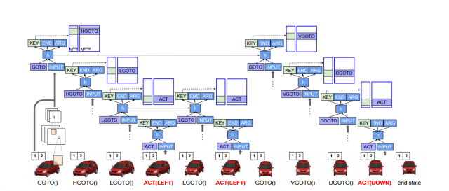
When the NPI is trained, the emitted low-level or high-level operation is compared to that produced by the actual program to be learned, and if they do not match, the NPI is penalized. Whenever NPI fails to properly predict the operation to be executed during training, there's a question whether we should execute in the environment the correct operation from the actual execution trace we are feeding, or the operation that the NPI predicted. The motivation behind executing the correct operation is that if we feed predicted operations (which early on during training are mostly meaningless), the error in the environment accumulates, and the NPI has no chance of predicting consecutive operations correctly. The motivation behind feeding the predicted operations is that after the NPI is trained, during evaluation it will always be fed the predicted operations (since the correct ones are not known), and so feeding the correct ones during training makes the model to be trained in a setting that is different from the setting in which it will be evaluated. While there's a good technique that addresses this issue called Scheduled Sampling, NPI doesn't use it, and always executes the correct operation in the environment during training, disregarding the predicted one.
In the original paper the NPIs are tested on several toy tasks, including the addition described above, as well as a car rotation problem where the input to the neural network is an image of a car, and the network needs to bring it into a specific state via a sequence of rotate and shift operations:

With both toy tasks NPI achieves nearly perfect success rate. However, NPIs are rather impractical, since one needs the execution traces to train them, meaning that one needs to write the program himself before being able to learn it. Other models such as Neural Turing Machines are more interesting from this perspective, since they can be trained from input-output pairs, so one doesn't need to have an already working program. I will talk about Neural Turing Machines, and their more advanced version Neural Differentiable Computer, in one of the next posts in this series.
Provably correct NPIs and Recursion
One of the problems with NPIs is that we can only measure the generalization by running the trained NPI on various environments and observing the results. We can't, however, prove that the trained NPI perfectly generalizes even if we observe 100% generalization on some sample environments.
For example, in the case of multidigit addition the NPI might internally learn to execute a loop and add corresponding digits, however over time a small error in its hidden state can accumulate and result in errors after many thousands of digits.
A new paper that was presented on ICLR 2017 called Making Neural Programming Architecture Generalize Via Recursion addresses this issue by replacing loops in the programs used to generate execution traces with recursion. Fundamentally nothing in the NPI architecture prevents one from using recursion -- during the execution of a high level operation A the LSTM can theoretically emit the same high level operation, or some other high level operation B that in turn emits A. In other words, the model used in the 2017 paper is identical to the model used in the original Scott Reed's paper, the difference is only in the programs used to generate the execution traces. Since in the new paper the execution traces are generated by programs that contain no loops, execution of any high level operation under perfect generalization should yield a bounded number of steps, which means that we can prove that the trained NPI has generalized perfectly by induction if we can show that it emits correct low level commands for all the base cases, and emits correct bounded sequences of high and low level commands for all possible states of relevant part of the environment.
For example, in the example of multidigit addition, it is sufficient to show that the NPI properly terminates when no more digits are available (the environment has no digits under cursors and CARRY is zero), and that the NPI correctly adds up two numbers and recurses to itself for any pair of digits under cursor and state of the CARRY. Authors of the paper show that for recursive addition algorithm an NPI trained only on examples up to five digits long provably generalizes for arbitrarily long numbers.
Hope it was interesting. In the next post I will switch from learning how to execute programs to learning how to write them, and will show a nice demo of a recurrent neural network that tries to predict next few tokens as the programmer writes a program.


