AlexLuchianov's blog

By AlexLuchianov, 2 years ago, In English

One advanced topic in competitive programming are flows. The main challenge in flow problems lays often not in the algorithm itself, but in modelling the graph. To solve the project selection problem, we will model it as an instance of the minimum cut problem:

"You are given a directed graph with weighted edges. One node is designated as a source and another as a sink. Erase a set of edges of minimal total weight such that the source and the sink become disconnected. The source and the sink are considered to be disconnected if there no longer exists a directed path between them"

The minimum cut problem is equivalent to the maximum flow problem. Note that we can consider the maximum flow problem as a black-box that solves our instances of minimum cut. Thus, once we manage to reduce our problems to minimum cut, we can consider them solved.

The project selection problem

This problems is most often stated as:

"You are given a set of $$$N$$$ projects and $$$M$$$ machines. The $$$i$$$-th machine costs $$$q_i$$$. The $$$i$$$-th project yields $$$p_i$$$ revenue. Each project requires a set of machines. If multiple projects require the same machine, they can share the same one. Choose a set of machines to buy and projects to complete such that the sum of the revenues minus the sum of the costs is maximized."

It is quite inconvenient that for projects we get revenue and for machines we have to pay, so let's assume that we are paid in advance for the projects and that we have to give the money back if we don't manage to finish it. These $$$2$$$ formulations are clearly equivalent, yet the latter is easier to model.

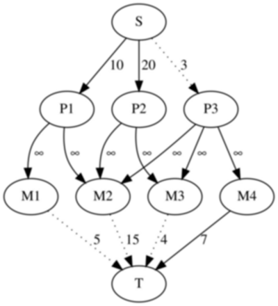
One simple way to model the above problem as a minimum cut is to create a graph with $$$N + M + 2$$$ vertices. Each vertex represents the source, the sink, a project or a machine. We will note the source as $$$S$$$, the sink as $$$T$$$, the i-th project as $$$P_i$$$ and the $$$i$$$-th machine as $$$M_i$$$. Then, add edges of weight $$$p_i$$$ between the source and the $$$i$$$-th project, edges of weight $$$q_i$$$ between the $$$i$$$-th machine and the sink, and edges of weight $$$\infty$$$ between each project and each of its required machines.

To reconstruct the solution, we will look at our minimum cut. If the edge between the source and the $$$i$$$-th project is cut, then we have to give the money back for the $$$i$$$-th project. If the edge between the $$$i$$$-th machine and the sink is cut, then we have to buy the $$$i$$$-th machine. It is easy to observe that for all dependencies between a project and a machine we will either buy the necessary machine or abandon the project since it would be impossible to cut the edge of weight $$$\infty$$$ between them.

An example of such a model

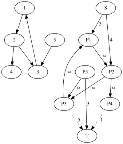
Our model can be extended even to dependencies between $$$2$$$ projects or between $$$2$$$ machines. For example, let's say that projects $$$i$$$ is dependent on the project $$$j$$$. To represent this restriction we can add an edge of weight $$$\infty$$$ from $$$i$$$ to $$$j$$$. In essence, this edge tells that we cannot abandon project $$$j$$$ without also abandoning project $$$i$$$. If machine $$$i$$$ is dependent on machine $$$j$$$ we will have to add an edge in the graph from machine $$$i$$$ to machine $$$j$$$. We can even add dependencies between a machine and a project. It is easily seen from this, that there is actually no difference between a machine and a project other than their costs, in essence a machine is simply a project that costs money.

One last detail is that in the case of a time paradox such as project $$$1$$$ requires project $$$2$$$, project $$$2$$$ requires project $$$3$$$ and project $$$3$$$ requires project $$$1$$$ we can accidentally take them all using our model. If that is alright, then there is no problem. Otherwise, if the projects should be done in order and not all at once, we have to eliminate from the graph all nodes that belong to a cycle.

This project selection problem can appear in many forms and shapes. For example, the machines and projects can also be represented as clothes and outfits or as some other analogies. In these cases, we can easily recognize the connection to our original problem and formulate a solution extremely fast. However, often the "machines and projects" will not be represented by simple objects, but by more abstract concepts.

The Closure Problem

"You are given a directed graph. Each node has a certain weight. We define a closure as a set nodes such that there exists no edge that is directed from inside the closure to outside it. Find the closure with the maximal sum of weights."

The problem above is known in folklore as the closure problem. The closure requirement can be reformulated as follows. For each edge $$$(x, y)$$$ if $$$x$$$ is in the closure then $$$y$$$ has to also be included into the closure.

It is easy to see that this problem and the project selection problem are closely related, equivalent even. We can model the inclusion of a node in the closure as a "project". The restrictions can also be easily modelled as dependencies between our projects. Note that in this case there is no clear line between machines and projects as usual.

Here is an example

This problem can also be disguised as open-pit mining. Once again, it is easy to see the connection between these $$$2$$$ problems. Here is a sample submission implementing this idea.

A more abstract example

"You are given a graph with weighted nodes and weighted edges. Select a valid subset of nodes and edges with maximal weight. A subset is considered to be valid if for each included edge, both of its endpoints are also included in the subset"

We can consider the nodes as 'machines' and the edges as projects. Now, it is easy to see an edge being dependent on its $$$2$$$ endpoints is equivalent to a project being dependent on $$$2$$$ machines.

This problem can be found here and a sample submission can be found here. If we didn't know about the project selection problem, then this problem would have been much harder.

An even more abstract example

"You are planning to build housing on a street. There are n spots available on the street on which you can build a house. The spots are labeled from $$$1$$$ to $$$N$$$ from left to right. In each spot, you can build a house with an integer height between $$$0$$$ and $$$H$$$.

In each spot, if a house has height $$$a$$$, you can gain $$$a^2$$$ dollars from it.

The city has $$$M$$$ zoning restrictions though. The $$$i$$$-th restriction says that if the tallest house from spots $$$l_i$$$ to $$$r_i$$$ is strictly more than $$$x_i$$$, you must pay a fine of $$$c_i$$$.

You would like to build houses to maximize your profit (sum of dollars gained minus fines). Determine the maximum profit possible."

Let's reformulate the restrictions. For a restriction $$$(l_i, r_i, x_i, c_i)$$$ We can assume that we will get punished for all of them and that we will get our $$$c_i$$$ dollars back if all of our buildings in the range $$$[l_i, r_i]$$$ are smaller than or equal to $$$x_i$$$. With this small modification, we can now only gain money.

Let the maximal height be $$$H$$$. Let's say that originally all buildings start at height $$$H$$$ and there are multiple projects to reduce them. For example, the project $$$(i, h)$$$ represents reducing the $$$i$$$-th from height $$$h$$$ to $$$h - 1$$$ for the cost $$$h ^ 2 - (h - 1)^2$$$. The project $$$(i, h)$$$ is clearly dependent on the project $$$(i, h + 1)$$$. Let's also add our restrictions as projects. A restriction $$$(l_i, r_i, x_i, c_i)$$$ is equivalent to a project with profit $$$c_i$$$ dependent on the projects $$$(l_i, x_i)$$$, $$$(l_i + 1, x_i)$$$ $$$\dots$$$ $$$(r_i, x_i)$$$. In less formal terms, this means that we can regain our money if we reduce the $$$l_i$$$-th, $$$l_i + 1$$$-th $$$\dots$$$ $$$r_i$$$-th buildings to height $$$h_i$$$.

Note that this problem could have also been solved using dynamic programming. However, our solution has the major advantage that it is more easily generalizable. For example, we can easily modify this solution to account for restrictions applied on a non-consecutive set of buildings.

This problem can be found here and a sample submission implementing this idea can be found here. The editorial of this problem also describes another approach using maximum flow, that is more or less equivalent to the one presented here.

Conclusion

The project selection problem is an useful tool when modelling problems. Of course, these problems can be directly modelled using the maximum flow problem, however it is easier to use this already existing method.

Please share other problems that can be reduced to the project selection problem or similar modellings.

Full text and comments »

  • Vote: I like it
  • +241
  • Vote: I do not like it

By AlexLuchianov, 2 years ago, In English

Both segment trees and dynamic programming are common topics in competitive programming. Sometimes, they even appear together. In this blog, we will mostly use segment trees as a black-box. As such, it is not necessary (though it is highly recommended) to know segment trees to understand this blog. Let's begin.

Longest Increasing Subsequence(LIS)

"You are given an array $$$v$$$ containing $$$N$$$ integers. Your task is to determine the longest increasing subsequence in the array, i.e., the longest subsequence where every element is larger than the previous one.

A subsequence is a sequence that can be derived from the array by deleting some elements without changing the order of the remaining elements."

This problem is most often solved using binary search. There are countless tutorials about this method, so I will not discuss it in detail. However, there exists a more general way to solve it using segment trees.

Since we only care about the order of the elements and not about the actual values we can normalize our array. By normalizing, I mean to transform an array while maintaining the comparison order of the elements. For example, $$$ [10, 23, 6, 23] $$$ can be normalized to $$$ [2, 3, 1, 3] $$$ . After normalization, all the elements will be in the range $$$[1, N]$$$. For more details about normalization check the sample code available at the end of this section.

Let $$$v_i$$$ be the $$$i$$$-th element of the array. We can start with a $$$O(N^2)$$$ simple solution using dynamic programming. Let $$$dp(i, j)$$$ be the length of the longest increasing subsequence consisting only of the first $$$i$$$ elements of the array and ending with the value $$$j$$$. The recurrence relation of $$$dp(i, j)$$$ has the following $$$2$$$ cases:

  • If $$$v_i = j$$$, then that means that we can try to add $$$v_i$$$ to our LIS. Thus, $$$dp(i, v_i) = max_{h < v_i}dp(i - 1, h) + 1$$$ .
  • Otherwise, our solution doesn't change by adding $$$v_i$$$ to the set of available elements, so $$$dp(i, j) = dp(i - 1, j)$$$ .

One way to implement this solution is to maintain a matrix $$$dp(i, j)$$$ and process it line by line, column by column. It would be highly inefficient to keep the whole matrix in memory at all times. Since the $$$i$$$-th line of the matrix depends only on the $$$i - 1$$$-th line of the matrix, let's try keeping in memory only the previous line and the current line. Note that this is a common trick to reduce memory usage in dynamic programming problems.

The final observation is that the line $$$i$$$ is extremely similar to line $$$i - 1$$$. In fact, they differ in at most one position. That position is $$$dp(i, v_i)$$$. It would be a shame to copy the whole line just to change one number in it, so let's keep in memory only one line and modify it accordingly. According to our recurrence, the value of $$$dp(i, v_i)$$$ is equal to one plus the maximum on the prefix $$$[1, v_i - 1]$$$. For an example of how those values change consider the array $$$v = [5, 2, 3, 2, 4, 1, 7, 6]$$$ and check out the following animation (Yellow means query on prefix, red means update on position):

Simulation of segment Tree

So, let's review, we need a data structure that allows us to both query the maximum on a prefix and update a value at a certain position. A simple segment tree is perfect for this job.

Here is the problem link and here is a sample submission.

LIS generalizations

The main advantage of using the segment tree solution over the binary search one is that it can easily be generalized to deal with more complex LIS generalizations. For example, we can also easily count the number of LIS-es. Note that sometimes more than one segment tree may be necessary:

"For a given sequence with $$$N$$$ different elements find the number of increasing subsequences with $$$K$$$ elements."

A straight-forward solution using dynamic programming would be to define $$$dp(i, j, h)$$$ as the number of increasing subsequences consisting only of the first $$$i$$$ elements of the sequence, having $$$j$$$ elements and ending with $$$h$$$. The recurrence can be split into the following $$$2$$$ cases:

  • We can try adding $$$v_i$$$ to the sequence, $$$dp(i, j, v_i) = dp(i - 1, j, v_i) + \sum^{v_i - 1}_{h = 1}{ dp(i - 1, j - 1, h)} $$$
  • Otherwise we can't really do anything with the current element, so $$$dp(i, j, h) = dp(i - 1, j, h)$$$ for all $$$h$$$ different from $$$v_i$$$

Once again, we could maintain a tridimensional-array, however that would be highly inefficient. We can observe that the elements with the first dimension $$$i$$$ depend only on elements with the first dimension $$$i - 1$$$. As before, we can reduce memory usage by maintaining only one matrix. We can also observe that since most of the time $$$dp(i, j, h)$$$ is equal to $$$dp(i -1, j, h)$$$, the elements in the matrix rarely change. Since the necessary operations are finding the sum on the prefix of a line and updating an arbitrary value in the matrix, we can maintain it using an array of segment trees. This allows us to solve the above problem in $$$O(NKlogN)$$$ time complexity and with $$$O(NK)$$$ memory.

This problem actually appeared in the past here on codeforces. Also, here is a sample submission.

More complex problems

Let's apply our new technique on some more complex problems. For example check out the following problem:

"You are given an array with $$$N$$$ white cells. You can pay $$$K$$$ coins to change the color of one cell. You can do this operation multiple times, however you must pay $$$K$$$ coins for each operation. At the end, you receive money based on $$$Q$$$ intervals. For each interval, you receive one coin for each distinct color present in it. (White counts as a color too).

You have to maximize the number of coins gained. "

A simple observation is that it does not make sense to paint over the same cell multiple times. Also, we will never reuse a color. After making these observations we can try to compute for each position its profit if we paint over it. We define the profit of a position as the number of intervals in which it is included minus $$$K$$$. A simple greedy would be to paint over all positions with positive profit.

However this strategy has a simple flaw. Since white is also considered a color, we can get an additional coin for each interval with at least one unpainted cell. Thus, sometimes it may not be optimal to paint a cell with a positive profit since it may already generate profit even as a white cell.

Let's adapt our problem statement to match our observations made so far:

"You are given an array with $$$N$$$ cells. Each cell has an associated profit $$$p_i$$$ if selected. There are also $$$Q$$$ intervals that reward us with $$$1$$$ coin if they have at least one unselected cell. Compute the maximal profit."

Now, the problem seems much easier to approach using dynamic programming. Let $$$dp(i, j)$$$ be the maximum profit if we consider only the prefix $$$[1, i]$$$ of the array and $$$j$$$ is the last not selected cell. Note that only intervals that are completely inside this prefix contribute to the profit. Instead of generating profit when selecting a cell, let's select all positions by default and pay $$$p_i$$$ when we decide to not select the $$$i$$$-th cell.

Let $$$f(i, j)$$$ be the number of intervals which end in $$$i$$$ and contain $$$j$$$. As earlier, the recurrence of $$$dp(i, j)$$$ can be split into the following $$$2$$$ cases:

  • We decide to not select the $$$i$$$-th position: $$$dp(i, i) = \max_{j < i} dp(i - 1, j) + f(i, i) - p_i $$$.

  • We decide to select the $$$i$$$-th position: $$$dp(i, j) = dp(i - 1, j) + f(i, j)$$$.

One can , once again, observe that the elements on the line $$$i$$$ depend only on line $$$i - 1$$$, so we could only use one line and modify it accordingly. However, one thing is different from the last time we did this. The lines can differ in multiple positions, they can even differ completely. Does this mean that it is impossible to further optimize this solution? The answer is no.

For now, let's ignore the existence of $$$f(i, j)$$$ when doing transitions:

  • We decide to not select the $$$i$$$-th position: $$$dp(i, i) = \max_{j < i} dp(i - 1, j) - p_i $$$.

  • We decide to select the $$$i$$$-th position: $$$dp(i, j) = dp(i - 1, j) $$$.

Now, this looks certainly more approachable. We can do this transition using segment tree. As for $$$f(i, j)$$$, it is actually the contribution of the intervals ending in $$$i$$$. Let's try not to add this contribution all at once using $$$f(i, j)$$$ and add them separately for each interval. What positions does an interval $$$(j, i)$$$ affect?. It actually only increases all positions $$$dp(i, j)$$$, $$$dp(i, j + 1)$$$ $$$\dots$$$ $$$dp(i, i)$$$ by $$$1$$$. Hmmm, so we only have to handle ranged updates that increase all elements in an interval with a fixed value and queries regarding the maximum value on some interval. This does sound a lot like segment tree with lazy propagation...

The most important aspect of this problem is the fact that sometimes, it is necessary to use more advanced variations of segment trees to solve them.

This problem can be found here. Unfortunately, it is on a Romanian website and its statement is not available in English. However, you can still use the website to submit your own solution to this problem. A sample submission implementing this approach that runs in $$$O((N + Q)logN)$$$ can be found here.

Obfuscation

Sometimes, the solution can be obfuscated under multiple layers of seemingly unrelated things. One extraordinary (quite underrated) example is the problem Colouring a rectangle from EJOI 2019 :

Statement of the problem

This problem seems unapproachable at first sight and completely unrelated to dynamic programming or segment trees. However, we only need to make some observations first.

Let's define LR-diagonals as diagonals that go from an upper-left position towards a lower-right position. In an analogue way, let's also define RL-diagonals as diagonals that go from an upper-right position towards a lower-left position. Also, note that we will index the rows and columns starting from $$$0$$$ and we will identify the element on row $$$i$$$ and column $$$j$$$ as $$$(i, j)$$$.

One known property of LR-diagonals is that $$$(i, j)$$$ and $$$(x, y)$$$ are on the same LR-diagonal if and only if $$$i - j = x - y$$$. RL-diagonals also have a similar property, namely $$$(i, j)$$$ and $$$(x, y)$$$ are on the same RL-diagonal if and only if $$$i + j = x + y$$$.

Since all elements in a LR-diagonal have a common invariant, let's use that invariant to identify diagonals. For example we will say that all elements $$$(i, j)$$$ make part of the LR-diagonal with id $$$i - j$$$. Similarly all elements $$$(i, j)$$$ also make part of the RL-diagonal with id $$$i + j$$$.

Thus, all LR-diagonals can be assigned an id ranging from $$$-(m - 1)$$$ to $$$(n - 1)$$$ and all RL-diagonals can be assigned an id ranging from $$$0$$$ to $$$(n - 1) + (m - 1)$$$.

Another interesting property of those diagonals is that LR-diagonals with even id's only intersect with RL-diagonals with even id's. The same is true for odd id's. An even more interesting property about the intersection of these diagonals is that all odd LR-diagonals intersect with a consecutive interval of odd RL-diagonals. The reverse is also true, all even LR-diagonals intersect with a consecutive interval of even RL-diagonals.

After all of these observations, we can finally start solving the problem. Since even diagonals don't intersect with odd diagonals, we can simply consider $$$2$$$ separate problems. Each element is at the intersection of a LR-diagonal and a RL-diagonal. This means that we have to color either the respective LR-diagonal or the respective RL-diagonal.

Let's choose a set of LR-diagonals to color, then color the necessary RL-diagonals. Since a RL-diagonal only intersects with a interval of LR-diagonals, the problem can be reformulated as follows:

"You are given an array with $$$N$$$ white cells. We can paint element $$$i$$$ for the price of $$$p_i$$$ coins. You are also given $$$Q$$$ restrictions. A restriction $$$(x_i, y_i, c_i)$$$ means that if the interval $$$[x_i, y_i]$$$ has at least one unpainted cell we have to pay an additional $$$c_i$$$ coins. Paint the array and fulfill all restrictions using a minimal number of coins"

One can easily see the connection between this problem and the original one. The array elements are the LR-diagonals and the restrictions are the RL-diagonals in disguise. This new problem seems much more approachable than the original.

From here on, we will simply do the same thing as in the previous problem. The only difference is that now we are actually punished for leaving an interval uncompleted, whereas previously we were rewarded for this.

Practice Problems

Conclusion

I hope you all liked this post. Also, if you know any additional problems or tricks related to this subject, please suggest them.

Full text and comments »

  • Vote: I like it
  • +278
  • Vote: I do not like it

By AlexLuchianov, 2 years ago, In English

The most common example when talking about sparse tables is the following problem:

"Given an array of $$$N$$$ integers, your task is to process $$$Q$$$ queries of the form: what is the minimum value in range $$$[a,b]$$$?"

A brute-force approach would be to iterate over all of the elements of each query interval. This approach has $$$O(NQ)$$$ time complexity and is quite slow. One way to improve the time complexity would be to precompute the minimum value for various intervals and then use this information to speed up the queries. For what intervals should we precompute the minimum value?

For a start, let's try precomputing it for all intervals of length $$$2$$$, $$$4$$$, $$$8$$$ and so on. More formally, let $$$rmq[h][i]$$$ be the minimum value on the interval $$$[i, i + 2^h - 1]$$$. One simple and efficient way to precompute this table is by observing that one interval whose length is a power of $$$2$$$ can be split into $$$2$$$ smaller intervals. This observation translates into the following recurrence relation: $$$rmq[h][i] = min(rmq[h - 1][i], rmq[h - 1][i + 2^{h-1}])$$$ . Below is an example of one such sparse table:

image

How can we actually use this to solve the queries? We could try splitting the queried interval into $$$logN$$$ disjoint intervals of length power of $$$2$$$. However, in this case we can do better. The $$$min$$$ operation is an idempotent operation. This may sound complicated, however this is simply a fancy math term for an operation that can be applied multiple times without changing the result beyond the initial application. Examples of common idempotent functions include: min, max, gcd, binary and, binary or.

The main advantage of these idempotent functions is that we no longer have to split the queries interval into disjoint intervals. Let $$$[a, b]$$$ be the queried interval and $$$P$$$ the largest power of $$$2$$$ that is smaller than or equal to the length of this interval. To find the minimum on $$$[a, b]$$$ we can simply look at the minimum on $$$[a, a + P - 1]$$$ and $$$[b - P + 1, b]$$$. Since $$$P$$$ is the largest power of $$$2$$$ that fits in $$$[a, b]$$$, these two intervals completely cover $$$[a, b]$$$.

To find the largest power of $$$2$$$ smaller than or equal to some value we can precompute it or simply use language-specific bit tricks. For example in C++ we can use the __builtin_clz function to count the leading zeros, then we can use this value to find the exponent of the largest power of 2 smaller than or equal to the original number. One thing to be careful of is that __builtin_clz(0) is undefined. Rust also has a function that counts the number of leading_zeros.

This allows us to solve the problem in $$$O(NlogN + Q)$$$ time complexity. The link to the problem can be found here and a link to a sample solution can be found here.

What if the function was not an idempotent one? In this case, we could have used disjoint sparse tables to achieve the same complexity. More about this topic can be found in the blog Video about Disjoint Sparse Table or how to answer all queries in constant time by peltorator (Unfortunately, the audio is in russian-only at the moment, however it has english subtitles). A text explanation about this topic can also be found here.

Regarding performance

One often forgotten detail is the fact that there is a time difference between using $$$rmq(h, i)$$$ and $$$rmq(i, h)$$$. This difference stems from the fact that $$$rmq(h, i)$$$ is cache-friendly. For example, see the following pieces of code:

  for(int h = 1; h <= lgmax; h++)
    for(int i = 1;i <= n - (1 << h) + 1; i++)
      rmq[h][i] = std::min(rmq[h - 1][i], rmq[h - 1][i + (1 << (h - 1))]);
  for(int h = 1; h <= lgmax; h++)
    for(int i = 1;i <= n - (1 << h) + 1; i++)
      rmq[i][h] = std::min(rmq[i][h - 1], rmq[i + (1 << (h - 1))][h - 1]);

To understand the performance difference of the above pieces of code, we first have to think about how memory is allocated in C++. A simple array is allocated in a contiguos memory block, but what about multidimensional arrays such as our rmq matrix. The short answer is that a matrix is also allocated this way by placing its lines one after another, thus transforming it into an array. How does this affect us? Let's say that we first access the element $$$rmq[h][i]$$$ and then $$$rmq[h][i + 1]$$$, since these locations in memory are close to each other we can go from one to another extremely fast. Now consider the elements $$$rmq[h][i]$$$ and $$$rmq[h + 1][i]$$$, these elements may seem extremely similar, however there is a whole matrix line between them. These memory jumps may seem inconsequential, but they too affect time efficiency.

Another advantage of $$$rmq[h][i]$$$ over $$$rmq[i][h]$$$ is that the former can be vectorized. In simple terms, this means that since the we apply the same transformation to a line of elements we can process multiple elements at once. Vectorization is something mostly done by the compiler.(In this case vectorization doesn't happen since the compiler cannot vectorize std::min). More information about this can be found in the blog About performance of sparse tables by sslotin.

Memory optimizations

If the queries are given in a offline manner (We receive all of the queries at the beginning) we can separate the queries into $$$logN$$$ groups. In the $$$i$$$-th group we will have the queries with lengths in the interval $$$[2^i, 2^{i + 1} - 1]$$$. To solve all of the queries in the $$$i$$$-th group we only need the minimums over all intervals of length $$$2^i$$$. The minimums over all intervals of length $$$2^i$$$ only depend on the minimum of all intervals of length $$$2^{i - 1}$$$. Thus, we can simply process the groups in increasing order while maintaining the minimums over all intervals of the corresponding power of $$$2$$$. This approach reduces memory to $$$O(N + Q)$$$, a sample submission implementing this idea can be found here.

One major downside to the above method is that the queries have to be given in an offline manner. We can sacrifice time efficiency to obtain a method that doesn't have this downside. A short explanation of one way to achieve this is the following. We can group the elements of the array in blocks of length $$$logN$$$, compress those blocks into an array of length $$$\frac{N}{logN}$$$ and compute a sparse table over this compressed array. We should also precompute the results for all prefixes/suffixes inside a block. To solve a query $$$[a, b]$$$, we have to consider two cases. First, if $$$a$$$ and $$$b$$$ are part of different blocks we can extract the answer by looking at the suffix of $$$a$$$'s block, at the prefix of $$$b$$$'s block and at the interval of complete blocks between $$$a$$$ and $$$b$$$. The suffixes and the prefixes are already computed and to extract information about the interval of blocks we can simply look into our sparse table over blocks. If $$$a$$$ and $$$b$$$ are in the same block we can simply iterate over all the elements in the interval $$$[a, b]$$$ in $$$O(logN)$$$ time complexity. Thus, the total time complexity is in the worstcase is $$$O(N + QlogN)$$$.

Note that a segment tree solution has the same complexity and that the only queries not solved in $$$O(1)$$$ are those completely included in blocks. In some cases, it is possible to optimize those queries to $$$O(1)$$$. An example of such a special case is the find minimum on interval operation. More information on this particular case can be found in the blog Range minimum query in O(1) with linear time construction by brunomont.

Reverse RMQ

One interesting modification is the reverse problem:

"You are given an array of $$$N$$$ elements. You have to process $$$Q$$$ updates $$$(x, y, val)$$$ which transform the array in the following way: For every position $$$i$$$ in the interval $$$[x, y]$$$, $$$v[i]$$$ becomes equal to $$$max(val, v[i])$$$. What is the array after all of the operations have been processed?"

This problem can easily be solved using Segment Trees in $$$O(N + QlogN)$$$. However, if $$$Q$$$ is significantly bigger than $$$N$$$ we can do better.

To solve this, we can use the same idea as before of using the intervals with length power of $$$2$$$. However, this time we will use those intervals to propagate information. Since the max operation is idempotent we can split each update interval into $$$2$$$ intervals with length power of $$$2$$$. Now, we can process the largest intervals by splitting them into $$$2$$$ smaller intervals and propagating the information forward. It may seem that each query contributes to the creating of $$$O(N)$$$ smaller interval, however since we only process intervals of length power of $$$2$$$ the total number of actually created intervals is $$$O(NlogN)$$$.

Thus, the total time complexity of this approach is $$$O(NlogN + Q)$$$. This problem can be found here and a sample solution here.

A more abstract application of reverse RMQ

Sometimes, this technique will be not be as obvious as previously. For example, check out the following problem:

"In this problem you are dealing with strings of length $$$N$$$ consisting of lowercase letters of the English alphabet. Each string should respect $$$M$$$ restrictions of the form:

  • $$$(len,x,y)$$$ the two substrings starting at $$$x$$$ and $$$y$$$, having a length of $$$len$$$, are equal.

Count the number of strings respecting all the $$$M$$$ restrictions. Print your answer modulo $$$10^9+7$$$."

A brute force approach would build a graph where each letter of the string is represented by a node and there is an edge between $$$x$$$ and $$$y$$$ if their corresponding characters have to be equal. Let $$$K$$$ be the number of connected components in this graph. Then, the number of valid strings is $$$26^K$$$. We can build such a graph in $$$O(NM)$$$, however that would be far too slow. We can observe that all $$$M$$$ restrictions can be split into $$$2$$$ equivalent restrictions of length power of $$$2$$$.

From here on, we can organize the restrictions into groups. The $$$i$$$-th group will contain all queries with length between $$$2^i$$$ and $$$2^{i + 1}-1$$$. We can process the restriction groups in decreasing order. For each restriction group there are only at most $$$O(N)$$$ relevant restrictions of the form substring $$$[x, x + 2^i - 1]$$$ is equal to substring $$$[y, y + 2^i - 1]$$$. (The other restrictions are irrelevant since they are implied). For each group we have to propagate our restrictions to the next group. For the group $$$i$$$ each restriction $$$(x, y)$$$ creates the restrictions $$$(x, y)$$$ and $$$(x + 2^{i - 1}, y + 2^{i - 1})$$$ for the group $$$i - 1$$$. To determine for each group what the relevant restrictions are we can use DSU. We can observe that we can reuse the same DSU for all groups since the restrictions of each group represent a superset of the restrictions of the previous groups.

The problem can be found here: Substring Restrictions and my solution can be found here. A similar approach is also discussed in its editorial.

Conclusion

I hope that you liked this blog and that you learned something useful from it. If you have any other sparse table tricks or problems, please share them.

Full text and comments »

  • Vote: I like it
  • +195
  • Vote: I do not like it

By AlexLuchianov, 2 years ago, In English

Some time ago, I was part of the scientific committee at infO(1)Cup. While discussing problems with other members of the committee I proposed the following problem:

You have to play a game against the interactor on a $$$N$$$ by $$$M$$$ matrix. Initially all cells are unclaimed. You and the interactor, alternatively, take turns claiming a non-empty set of unclaimed cells. The set of cells chosen in a turn has to be able to fit in a $$$K$$$ by $$$K$$$ bounding box without being rotated and has to be connected. (There exists a path between any two cells in the set passing only through cells in the set, we define a path as a sequence of cells such that any two consecutive cells have a common side). You can choose whether to play first or second.

Before I discuss the solution to the above problem, I first wish to show you a similar puzzle known in the folklore as "The round table coin game" or as "The faustian round table coin game" . The puzzle goes as follows:

The Devil proposes to play a game against you. If you win, he will give you everything that you desire, otherwise he will take your soul. The game is played on an empty round table. You take turns placing identical coins on the table. In a turn you have to place exactly one coin on the table such that it does not overlap with another one. Note that once a coin is placed on the table you can't move it. The player who cannot make a move loses. You can choose whether to play first or second.

The winning strategy is to choose to play first and place a coin in the center of the table. Then, you can always mirror the opponents move as follows:

Coin

As seen in the animation above we will never run out of moves to do, since our opponent has to do them first. Now, let's return to our original task. We can try extending this reasoning by considering the following 2 cases:

  • If $$$K$$$ is $$$1$$$, there is not much that we can do since all players can only claim exactly one cell per turn. We can decide whether to go first or second by looking at the total number of moves $$$N * M$$$. If it is odd, we should play first. Otherwise, we should play second.

  • Otherwise, we could try transforming our coin strategy to adapt to this setting. We start by placing a $$$1$$$ by $$$1$$$ square in the middle of the board and then mirror our opponents moves. Unfortunately, this strategy has two major flaws.

First, let's consider a board with even lengths. Where exactly is the center and how can we place a $$$1$$$ by $$$1$$$ square there? The answer is that the center is in this case not a $$$1$$$ by $$$1$$$ square but a $$$2$$$ by $$$2$$$ square, so we have to adapt our strategy to place $$$2$$$ by $$$2$$$ squares. What about boards with even length and odd width or vice versa? For them, the center is not a square, but actually a $$$1$$$ by $$$2$$$ or $$$2$$$ by $$$1$$$ rectangle. Naturally, we should adapt our strategy to consider such cases and if necessary place rectangles instead of squares in the middle.

Secondly, if in the first turn we play a piece that is too small, our opponent could place a really long piece that wraps around our middle piece and intersects with its own mirror image. This flaw can be easily corrected by making the middle piece as big as possible while still respecting the bounding box condition and its symmetry.

After correcting these $$$2$$$ flaws, we finally have a working strategy. Check out the following animation for an example:

Tetris

How do we actually write the interactor?

The strategy of the contestant should be clear now, but what about the strategy of the interactor? How can we guarantee that a wrong solution will fail? If the contestant chooses to play as the second player, we can easily punish them by making the grader play perfectly as the first. If the first player places a middle piece that is too small, we can simply wrap around it, thus creating a bigger middle piece. However, what if our opponent decides to not even place his first piece in the middle? Or what if our opponent places the first piece correctly, but fails to mirror our moves. How can we punish such incorrect solutions?

After careful consideration, we reached the conclusion that the only way to punish the contestant for having a bad strategy was to do random moves until the end. We claimed that if the contestant had a bad strategy, then by doing those random moves we could create enough chaos on the board to derail his algorithm and balance our chances of winning. Those random moves would be mostly spread around the sensitive spots such as the center or the mirror images of already placed pieces. This is a decent method since the interactor only has to win once to deem the solution incorrect, while the contestant has to win all the time.

Another idea that was proposed during the meeting was that if we restricted to the shape of the sets of cells it would be easier to come up with a strategy for the interactor to punish those wrong moves. The discussed shapes included but were not limited to: only squares, only rectangle, only tetris pieces. We even considered introducing non-connected shapes, however none of these ideas materialized into something useful.

In the end, the question boiled down to the 2 following points:

  • Is it acceptable to propose such an interactive problem if you can't guarantee that the judge will play optimally well? And if it is acceptable, where do we draw the line? What is the acceptable probability of an incorrect strategy passing?

  • Should we even invest that much time into preparing this problem? Or as a very wise man once said: "Is it even worth to propose a problem if the grader is harder to write than the actual solution?".

Ultimately, the problem didn't make the cut because of all of these shortcomings. However, that is exactly why it is worth sharing here.

Open questions

  • Do we have a name for this type of game theory problems, where there exists an easily provable winning strategy for the first move, yet it is almost impossible to determine for an arbitrary state if it is winning?
  • Is there any modification of the problem, for which it is possible to find a strategy for the interactor?
  • Is there any strategy that the first player can adopt that will win against a random interactor, yet will lose against a hypothetical perfect player?

Closing remarks

I wish to thank awoo, Ari, and -is-this-fft- for helping me with making the animation work on codeforces. For any future persons that wish to upload animations, use the .gif format and upload it with the .png extension (Just change the extension, don't change the format to .png). I also wish to thank my brother for doing the animations.

In any case, I hope you liked this blog and I hope to hear your opinion regarding such problems.

Full text and comments »

  • Vote: I like it
  • +207
  • Vote: I do not like it

By AlexLuchianov, 2 years ago, In English

"I used to be a competitive programmer like you, but then I took a macro to the knee."

First I want to say that I recognize the fact that not all macros are bad, there are even some ingenious macros that are really useful such as the all(x) macro from the post C++ tips and tricks by Golovanov399 . Another useful macro is NDEBUG. This macro is used to disable all assertion checks inside the code. It can be used like this:

#define NDEBUG
#include <cassert>

Note that NDEBUG has to be defined before including cassert to have an effect. Other useful macros are the debug macros, a little more information about them can be found in the following blog, Compilation and debugging tutorial by ramchandra.

However, for every one such great macro there exist another countless macros that are, let's just say, not that great. Here are some reasons for which I believe that macros should be used only with great care.

Macros ignore namespaces

One problem with macros is the fact that they completely ignore namespaces, for an example check the following code below:

#include <iostream>
namespace a {
  #define f(x) (x * 2)
};
namespace b {
  #define f(x) (x * 3)
};
int main() {
  std::cout << a::f(2) << '\n';
  return 0;
}

This code will not compile since macros are, in reality, just text substitutions handled by the pre-processor which does not know anything about namespaces or classes. In a small project this may seem like a minor inconvenience since you can simply remember what macros you have used. However, in a large project with many dependencies, this can create a massive amount of headaches for those involved. That is why it is recommended to undefine the macros at the end of the file in which they are defined, so that they do not affect other files.

Of course, this argument doesn't really apply to competitive programming since most contests are individual contests and the projects are small.

Macros reduce code readability

There is also the issue of readability. I often see codes full of weird for macros such as the following:

#define f0r(a, b) for(int i = a; i <= b;i++)
#define f0rr(a, b) for(int i = a; b <= i;i--)

These macros make the code, to say the least, unreadable for someone not used to this specific type of macro. In real projects where multiple people work together this will make teamwork extremely hard. Once again, this is competitive programming and if you understand your own code that is all that matters. I also wish to say that, although I do not encourage the use of macros, I understand that some people value efficiency and will prefer to write shorter less readable code.

Most macros also have better modern alternatives

For example, let's consider the popular #define ll long long has the much better alternative using ll = long long. The main difference is that the latter variant allows us to write things such as ll(a) to convert the result into a long long, whereas this doesn't compile if using define.

Some people also use macros to define constants like #define INF 1000000000, however we can also use the alternative: int const INF = 1000000000;. The advantages of using constants instead of macros include type-safety checking and respecting namespaces.

Another macro that I often see is #define int long long. This is often done to quickly solve problems involving overflows. However, this is both bad practice and can potentially affect execution time negatively if the judge is using a 32-bit system.

Macros are not functions

A piece of code is worth a thousand words, so try to guess the output of the following piece of code:

#include <iostream>
#define plustwo(x) x + 2
int main() {
  std::cout << plustwo(2) * 3 << '\n';
  return 0;
}

One would guess that the output of the code above is $$$12$$$, however the actual output is $$$8$$$.

Why does this happen? Did the compiler make an error when processing this code? The answer is that the compiler worked just as intended. Let's examine in more detail what #define plustwo(x) x + 2 actually does. This define searches for occurrences of plustwo(x) and puts in their place x + 2. So, the code above is actually equivalent to:

#include <iostream>
int main() {
  std::cout << 2 + 2 * 3 << '\n';
  return 0;
}

Now, it is clear what the output is supposed to be. One quick fix is to pad the macro with parentheses as follows: #define plustwo(x) ((x) + 2).

Unfortunately padding does not solve all of our problems. For example, see the following code:

#include <iostream>
#define square(x) ((x) * (x))
int main() {
  int x = 2;
  std::cout << square(x++) << '\n';
  return 0;
}

It's output is $$$6$$$. Why does this happen even though we padded everything? The reason is that the code above translates to the following:

#include <iostream>

int main() {
  int x = 2;
  std::cout << ((x++) * (x++)) << '\n';
  return 0;
}

No matter how we look at the code above, it is obvious that some strange things are happening inside. One thing that makes this situation even worse is the fact that the order of evaluation is also undefined. The general rule of thumb to avoid such headaches is to not use more than one x++ or ++x in a single operation.

So, if we pad our macros and we don't mix it with x++ or ++x, are we actually safe? The answer is, unfortunately, no.

The most evil macro of all

The worst macros of all are, undoubtedly, the MIN and MAX macros. First we must understand why do people actually use them if we have modern alternatives such as std::min and std::max. This issue was actually also discussed here. The short answer is that people used those macros because it didn't check for equal types and it was marginally faster than the std alternatives. I'm not going to lie, I actually used those macros too exactly because of those reasons. I discovered after some time how dangerous they actually are, so I stopped using them. The program below is a clear illustration of the risk of using these macros:

#include <iostream>

#define MIN(a, b) (((a) < (b)) ? (a) : (b))
#define MAX(a, b) (((a) < (b)) ? (b) : (a))

int const nmax = 20;
int v[5 + nmax];
int step = 0;

int f(int n) {
  ++step;
  if(n == 1)
    return v[n];
  else
    return MAX(f(n - 1), v[n]);
}

int main() {
  int n = 20;
  for(int i = 1; i <= n; i++)
    v[i] = n - i + 1;
  step = 0;
  std::cout << f(n) << " ";
  std::cout << step << " ";

  return 0;
}

The output of the code above is 20 1048575. Why does the function make such a big number of steps? To find the answer we must look at how the function actually looks after we process the MAX keyword:

int f(int n) {
  ++step;
  if(n == 1)
    return v[n];
  else
    return (((f(n - 1)) < (v[n])) ? (v[n]) : (f(n - 1)));
}

What the ternary operator actually does is compute $$$f(n - 1)$$$ and it then compares it with $$$v[n]$$$. Then since $$$f(n - 1)$$$ was bigger and the expression f(n - 1)) < (v[n]) is true it decides to return $$$f(n - 1)$$$. Thus, it has to evaluate $$$f(n - 1)$$$ again. Note that if we initialized array $$$v$$$ with increasing numbers instead of decreasing numbers the program would have made only $$$20$$$ steps and we would have never noticed this vulnerability. The bug would be even harder to detect if we used the MIN/MAX macros in, let's say, a Segment Tree implementation(This actually happened to me once).

Conclusion

Most times macros have modern safe alternatives. Nonetheless, in some cases macros are really useful, thus we should not be afraid to use them. Please share your favorite macros or share some stories about your worst macros:)

Full text and comments »

  • Vote: I like it
  • +280
  • Vote: I do not like it

By AlexLuchianov, 2 years ago, In English

The classic Problem

The most common application of binary lifting is the following:

"Let $$$G$$$ be a rooted tree with $$$N$$$ nodes. For $$$Q$$$ queries of the form $$$(K, V)$$$ we want to find the $$$K$$$-th ancestor of $$$V$$$ in the tree."

One simple, yet quite inefficient way of solving this problem is to build for every node an edge towards its direct ancestor. Then, in order to solve a query we simply have to traverse $$$K$$$ edges. This approach has complexity $$$O(NQ)$$$. We can try improving it by adding some "jump-edges".

Fig 1

A jump-edge is simply an edge that starts from a node and is not directed towards its parent, but towards an arbitrary ancestor. These jump-edges will allow us to traverse large regions of edges in a single operation. Let's start by building jump-edges from each node towards its $$$2$$$-nd ancestor, $$$4$$$-th ancestor, $$$8$$$-th ancestor and so on. Note that in the above figure only a subset of these jump-edges is visible since otherwise it would clutter the image too much.

Let's define the length of a jump-edge as the number of normal edges that are skipped by traversing this jump-edge. For example, all the blue edges in the above figure have length 4. We can compute the destination of these jump-edges in a recursive manner by using already computed shorter edges.

More formally, we denote $$$far(h, i)$$$ = the $$$2^h$$$-th ancestor of $$$i$$$. This can be calculated easily using the following recurrence $$$far(h,i) = far(h - 1, far(h - 1, i))$$$. Now to find the $$$K$$$-th ancestor we can greedily traverse the longest jump-edge that doesn't pass the $$$K$$$-th ancestor. We can do this by splitting $$$K$$$ into powers of $$$2$$$ and then traversing the edges of corresponding lengths in order. For example, let's search for the $$$7$$$-th ancestor of $$$9$$$. Since $$$7$$$ = $$$4$$$ + $$$2$$$ + $$$1$$$, we can traverse the blue edge from $$$9 \to 5$$$, the red edge from $$$5 \to 3$$$ and the black edge from $$$3 \to 2$$$.

This approach has time complexity $$$O((N+Q)log_2N)$$$ and memory complexity $$$O(Nlog2N)$$$.

Link to the above problem and to a submission implementing this solution.

Can we do better?...

In this particular case, we can exploit the fact that the queries are given in an offline manner (We can read all queries at the beginning and solve them together). We will explore the tree using a DFS and we will maintain in an array all of the ancestors of the current node (including itself). To maintain this array of ancestors we can simply do the following: When going from a node to its son we push the son to the end of this ancestor array and when returning from a node to its father we remove it from the end of the ancestor array. As such, when we reach a node we can easily answer the queries related to it by accessing the array of ancestors. Code implementing this idea can be found here.

However, what could we do if we first had to answer a query before getting the next one? Unfortunately, in this case we are not able to improve the time complexity further than $$$O((N + Q)log_2N)$$$, however we can reduce the required memory.

One way of reducing the required memory so is to sacrifice time efficiency and change the base of the length of the jumps. Instead of precomputing jump-edges with power of $$$2$$$ lengths, we can precompute jump-edges of lengths that are powers of another integer $$$D$$$. Using this method we have time complexity $$$O((N + Q)Dlog_DN)$$$ and memory complexity $$$O(Nlog_DN)$$$. This may not seem like that much of an improvement, though I have used it time and again to fit unintended solutions in problems with extremely tight memory limits. A solution implementing this idea can be found here.

...without sacrificing execution time?

We can reduce memory to $$$O(N)$$$ without massively impacting the execution time. We can compute for each node its direct ancestor and a single jump-edge towards an arbitrary ancestor. When searching for the $$$K$$$-th ancestor we will try to traverse the jump-edge if it does not pass over the $$$K$$$-th ancestor, just like before. One way to choose the destination of these jump edges can be observed in the following picture:

Fig 2

Let's denote the direct ancestor of $$$x$$$ as $$$parent_x$$$. We will add jump-edge $$$x \to y$$$ only if the jump-edges from $$$parent_x \to z$$$ and $$$z \to y$$$ exist and have the same length for an arbitrary $$$z$$$. It is easy to see that we can compute all such jump-edges in $$$O(N)$$$ by processing the tree from top to bottom.

What is not so easy to see is why we can reach the $$$K$$$-th ancestor in logarithmic time by using these edges. The proof for this is quite long and uses skew-binary number systems, as such I will leave it as an exercise to the reader:) ( A bound of $$$3 \lfloor \lg(N + 1) \rfloor -2$$$ is shown in the original paper An applicative random access stack)

Source code implementing this approach can be found here.

Another way to do this is to choose $$$\frac{N}{logN}$$$ arbitrary nodes and create from them a virtual tree where there is an edge between $$$x$$$ and $$$y$$$ if $$$x$$$ is an ancestor of $$$y$$$ and there are no other chosen nodes on the path between them. We can compute jump-edges in this virtual tree using $$$O(\frac{N}{logN} * logN) = O(N)$$$ memory. To answer a query we find our closest ancestor that is part of this virtual tree and walk up to it (This ancestor is expected to be at a distance of around $$$logN$$$ edges since we chose the virtual tree nodes randomly). From here, we can use the jump-edges from the virtual tree to get as close to our $$$K$$$-th ancestor as possible. After there are no more jump-edges that we can use, we can return to using the edges from the original tree, since our target is expected to be at a distance of only around $$$logN$$$ edges.

Thanks to FairyWinx for suggesting this idea and I am extremely happy to see a nondeterministic method of achieving $$$O(N)$$$ memory. Here is a submission implementing this approach.

Computing the lowest common ancestor using binary lifting

Another common application of binary lifting is computing the lowest common ancestor(from now on we will abbreviate it as LCA) of $$$2$$$ nodes. In addition to precomputing our jumps-edges we should also compute for each node its depth. For simplicity, let's assume that we are using the original method to create jump-edges (the one using powers of 2). Let $$$x$$$ and $$$y$$$ be $$$2$$$ nodes to find their LCA we can apply the following strategy:

  1. Let's assume that $$$depth_y \le depth_x$$$, otherwise we can just swap them.

  2. Let $$$K = depth_x - depth_y$$$ and $$$z$$$ be the $$$K$$$-th ancestor of $$$x$$$ The LCA of $$$x$$$ and $$$y$$$ is the same as the LCA of $$$y$$$ and $$$z$$$, since the depth of the LCA is at most the depth of $$$y$$$ that is equal to the depth of $$$z$$$. We can substitute $$$x$$$ by $$$z$$$ and from now on assume that $$$depth_x = depth_y$$$.

  3. If $$$x = y$$$ we can stop since their LCA is clearly $$$x$$$. If the direct ancestor of $$$x$$$ is equal to the direct ancestor of $$$y$$$, we can also stop since that direct ancestor is their LCA. Otherwise, let $$$K$$$ be the highest power of $$$2$$$ lower than or equal to $$$depth_x$$$. If the $$$K$$$-th ancestor of $$$x$$$ and the $$$K$$$-th ancestor of $$$y$$$ differ, then we can reduce the problem to finding the LCA of the $$$K$$$-th ancestor of $$$x$$$ and the $$$K$$$-th ancestor of $$$y$$$. Otherwise, if the $$$K$$$-th ancestors are the same, then from now on we should only consider smaller jumps.

The $$$O(N)$$$ memory approach is also compatible with LCA queries. The steps $$$1$$$ and $$$2$$$ are identical, as for step 3 since $$$depth_x = depth_y$$$ their only jump-edges have the exact same length $$$K$$$, so we can check if they lead to the same node or not. If they do not, then we can reduce the problem to finding the LCA of their $$$K$$$-th ancestors. Otherwise, we can reduce the problem to finding the LCA of their parents.

Link to a problem that asks for the lowest common ancestor and source code implementing this approach can be found here with $$$O(N\log_2N)$$$ memory and here with $$$O(N)$$$ memory.

Path aggregates using binary lifting

Another useful application of binary lifting is extracting information about paths on trees. For example, the following problem can be solved using binary lifting:

"Let $$$T$$$ be a tree with weights on the edges. For $$$Q$$$ queries $$$(x, y)$$$ we want to find the maximum weight of the edges on the path from $$$x$$$ to $$$y$$$"

To solve this problem we can maintain additional information on the jump-edges such as the maximum over all of the normal edges that are passed by this jump-edge. To extract the maximum weight on a chain $$$(x, y)$$$, we will first define $$$z$$$ as the LCA of $$$x$$$ and $$$y$$$ and split the path $$$x \to y$$$ into $$$x \to z$$$ and $$$z \to y$$$. To find the maximum on the path $$$x \to z$$$ we can simply split it into jump-edges, just like before, and compute the maximum over all of these jump-edges.

Unfortunately, binary lifting can't be extended to cases where the weights of the edges are updated or the structure of the tree is affected. For the former it is necessary to use heavy light decomposition, as for the latter it is necessary to use link cut tree. These algorithms are quite long and tedious to implement, so it is preferable to use binary lifting when possible.

Since I could not find a problem that asked for this directly, here is one that can be reduced to this and here is code implementing this idea.

Additional problems

Conclusion

I hope you all liked this article and I encourage you to share problems that can be solved using this technique and maybe additional tricks related to it that I have missed. Thanks for all of your suggestions:)

Full text and comments »

  • Vote: I like it
  • +291
  • Vote: I do not like it