If I was a YouTuber, this would be the place where I fill the entire screen with screenshots of people asking me to make this. Anyway, not so long ago I gave a lecture on FFT and now peltorator is giving away free money, so let's bring this meme to completion.
In this blog, I am going to cover the basic theory and (competitive programming related) applications of FFT. There is a long list of generalizations and weird applications and implementation details that make it faster. Maybe at some point I'll write about them. For now, let's stick to the basics.
The problem. Given two arrays $$$a$$$ and $$$b$$$, both of length $$$n$$$. You want to quickly and efficiently calculate another array $$$c$$$ (of length $$$2n - 1$$$), defined by the following formula.
$$$c_k = \displaystyle \sum_{i + j = k} a_i \cdot b_j.$$$Solve it in $$$O(n \log n)$$$.
First of all, why should you care? Because this kind of expression comes up in combinatorics all the time. Let's say you want to count something. It's not uncommon to see a problem where you can just write down the formula for it and notice that it is exactly in this form.
FFT is what I like to call a very black-boxable algorithm. That is, in roughly 95% of the FFT problems I have solved, the only thing you need to know about FFT is that FFT is the key component in an algorithm that solves the problem above. You just need to know that it exists, have some experience to recognize that and then rip someone else's super-fast library off of judge.yosupo.jp.
But if you are still curious to learn how it works, keep reading... $$$~$$$
The strategy
By the way, the array $$$C$$$ we are calculating is called a convolution of $$$A$$$ and $$$B$$$. There are other kinds of convolutions, but this is the kind we care about here. Anyway, does the expression for $$$C$$$ remind you of anything?
Polynomials! Imagine that the arrays $$$A$$$ and $$$B$$$ were the coefficients of some polynomials.
$$$ \begin{align*} A(z) &= a_0 z^0 + a_1 z^1 + \cdots + a_{n - 1} z^{n - 1}, \\ B(z) &= b_0 z^0 + b_1 z^1 + \cdots + b_{n - 1} z^{n - 1}. \end{align*} $$$If we look at things this way, what would $$$c$$$ represent? It turns out that $$$c$$$ is exactly the coefficients of the polynomial $$$C(z) = A(z) \cdot B(z)$$$. If you don't see why, I recommend you write the multiplication out with pen and paper. By the way, I am denoting the variable with $$$z$$$ here because we are going to work with complex numbers, and it is customary to write complex variables as $$$z$$$ instead of $$$x$$$.
Crash course on complex numbersThis blog and this algorithm heavily depend on complex numbers. You may notice that I'm about to start using $$$j$$$ as an index everywhere, because annoyingly $$$i$$$ is taken. I'm not going to comprehensively teach complex numbers from scratch, but just to remind you, here are some facts.
There is no real number $$$x$$$ such that $$$x^2 = -1$$$. It is possible to expand the set of real numbers by introducing such a number $$$i$$$. The complex numbers are this set and consist of all numbers of the form $$$a + bi$$$, where $$$a$$$ and $$$b$$$ are real numbers. This is not the formal definition of complex numbers because this is not a formal introduction to complex numbers.
Basic arithmetic operations can be performed on the complex numbers by applying the usual rules:
- $$$(a + bi) + (c + di) = (a + c) + (b + d)i$$$.
- $$$(a + bi) (c + di) = ac + adi + bic + bdi^2 = (ac - bd) + (ad + bc)i$$$.
One can imagine a complex number $$$a + bi$$$ as a point (or vector) in a two-dimensional plane. $$$a$$$ is its $$$x$$$-coordinate and $$$b$$$ is its $$$y$$$-coordinate. Adding two complex numbers is then just like adding two vectors.
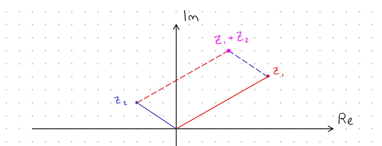
This also gives rise to an alternative way to think about a complex number: imagine it as a vector and consider its length and the angle between it and the real axis. The length and the angle are called the modulus and the argument, respectively. A complex number is uniquely defined by these two attributes. This also allows us to conceptualize the product of two complex numbers. When two complex numbers are multiplied, their moduli are multiplied and their arguments are added.

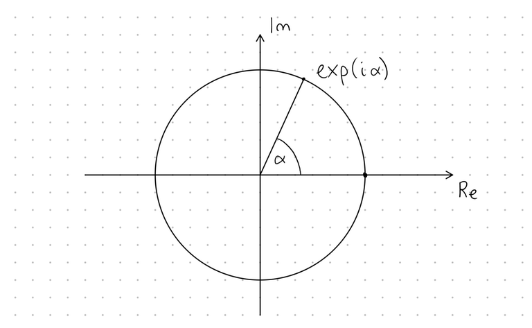
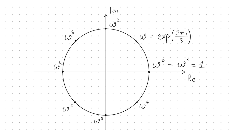
The set of complex numbers with modulus 1 form the unit circle. A very useful function is $$$f(\alpha) = e^{i \alpha}$$$, also written $$$\exp(i \alpha)$$$. Given a real number $$$\alpha$$$, $$$\exp (i \alpha)$$$ is always on the unit circle. As $$$\alpha$$$ increases, $$$\exp (i \alpha)$$$ moves counterclockwise in an uniform pace around the unit circle, reaching full circle at $$$\alpha = 2 \pi$$$. In other words, $$$\exp (i \alpha)$$$ is the unique complex number at the unit circle, at an $$$\alpha$$$-radian angle with the real axis. In particular, $$$e^{i \pi} = -1$$$.
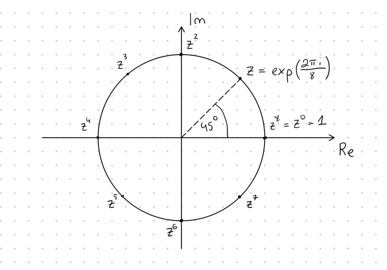
For example, $$$z = \exp \left( \frac{2 \pi i}{8} \right)$$$ is on the unit circle, at a 45-degree angle with the real axis. Its powers go along the unit circle with 45-degree steps: $$$z^2$$$ is at a 90-degree angle, $$$z^3$$$ at a 135-degree angle and so on. In particular $$$z^8 = 1$$$.
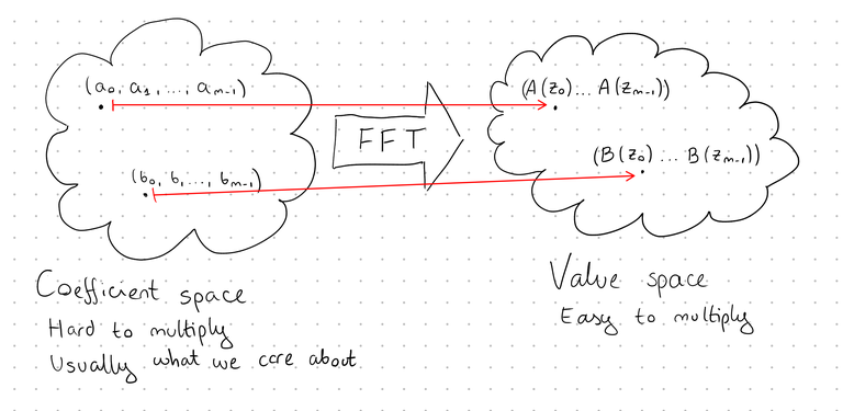
So, we now know that we want to multiply two polynomials. But how does that help us? For one, imagine if we, instead of the coefficients of $$$A$$$ and $$$B$$$, knew the values of $$$A$$$ and $$$B$$$ for a number of fixed $$$z$$$. That is, we have decided on some numbers $$$z_0, z_1, z_2, \ldots, z_{m - 1}$$$ and know all of the following:
$$$ \begin{align*} A (z_0), A (z_1), A (z_2), &\ldots, A (z_{m - 1}) \\ B (z_0), B (z_1), B (z_2), &\ldots, B (z_{m - 1}) \end{align*} $$$Finding the same values for $$$C$$$ is now dead simple. We just calculate $$$C (z_0)$$$ as $$$A (z_0) \cdot B (z_0)$$$, $$$C (z_1)$$$ as $$$A (z_1) \cdot B (z_1)$$$ and so on.
Also, knowing the values of a polynomial is not worse than knowing its coefficients. Knowing the value of a polynomial $$$C(z)$$$ for sufficiently many different $$$z$$$ is enough information to find out what the coefficients of $$$C$$$ are.
Fact. Given $$$m$$$ pairs $$$(z_0, w_0), (z_1, w_1), \ldots, (z_{m - 1}, w_{m - 1})$$$ where all the $$$z$$$-s are distinct, there is exactly one polynomial $$$P$$$ with degree up to $$$m - 1$$$ such that $$$P(z_i) = w_i$$$ for each $$$i$$$.
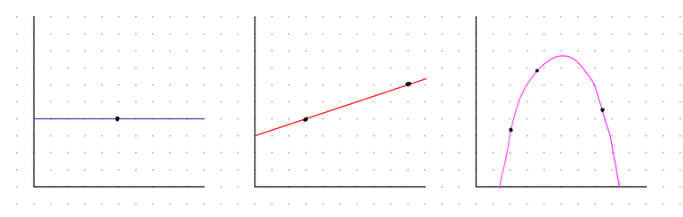
For example:
- given a point on a plane, there is exactly one way to draw a horizontal line (i.e. a constant polynomial) through it.
- given two points on a plane with different $$$x$$$-coordinates, there is exactly one way to draw a line (i.e. linear polynomial) through them.
- given three points on a plane with different $$$x$$$-coordinates, there is exactly one way to draw a parabola (i.e. quadratic polynomial) through them.
If you know the coefficients of polynomials, it is easy to add them, but hard to multiply them. To efficiently multiply polynomials, we need to know the values of polynomials. However, the coefficients of polynomials are what we are usually (maybe indirectly) given, and often also what we need to work with after multiplying. Therefore, we need a bridge between them. An algorithm that can quickly transport you from coefficient-world to value-world. That algorithm is the fast Fourier transform.
It should be noted that FFT doesn't calculate the values of the polynomial for arbitrary $$$z_0, \ldots, z_{m - 1}$$$, but rather one specific set.
The core of the algorithm
Now we are ready to tackle the hard part. We're given a polynomial $$$A(z) = a_0 z^0 + \cdots + a_{m - 1} z^{m - 1}$$$. First, let's make life easier for us and assume $$$m$$$ is always a power of two, say $$$2^k$$$. It can't hurt and we can easily do so by appending zeros to the end of the array of coefficients. Anyway, we need to calculate the value of $$$A(z)$$$ for $$$n$$$ distinct $$$z$$$-s.
Which $$$z$$$-s? We haven't decided yet, and we only need one set. It is pretty clear that we need to make the choice carefully, and that the algorithm will need to exploit some special properties of these values. But the crash course above hints at the correct choice, so I'm just going to make it. Hopefully it will become clear why. I define
$$$z_j = \exp \left( \frac{2 \pi i j}{m} \right).$$$The numbers $$$z_0, z_1, z_2, \ldots, z_{m - 1}$$$ go along the unit circle of the complex plane, evenly spaced apart. It gets better. If I define $$$\omega = z_1 = \exp\left(\frac{2 \pi i}{m}\right)$$$, then $$$z_j = \omega^j$$$. Convenient. These numbers have a neat property: $$$\omega^0 = \omega^m = 1$$$, $$$\omega^1 = \omega^{m + 1}$$$ etc. The exponents behave as though we are adding them, modulo $$$m$$$. $$$\omega$$$ is an omega, not a double-u.
Definition. Given an array $$$a_0, a_1, \ldots, a_{m - 1}$$$, the fast Fourier transform is any algorithm that calculates the tuple $$$(A(\omega^0), A(\omega^1), \ldots, A(\omega^{m - 1}))$$$ in $$$O(m \log m)$$$ time. The transform itself is called the discrete Fourier transform. We denote
$$$\mathrm{DFT}(a_0, a_1, \ldots, a_{m - 1}) = (A(\omega^0), A(\omega^1), \ldots, A(\omega^{m - 1})).$$$Now let's explain one possible FFT algorithm. This is the most well-known one, also known as the Cooley-Tukey algorithm. It is convenient to explain the algorithm by doing basic matrix operations, so let's translate the problem to matrix form. Given $$$a_0, a_1, \ldots, a_{m - 1}$$$, we need to calculate $$$A(\omega^0), A(\omega^1), \ldots, A(\omega^{m - 1})$$$. In matrix form, this means calculating
$$$ \begin{bmatrix} \omega^0 & \omega^0 & \omega^0 & \cdots & \omega^0 \\ \omega^0 & \omega^1 & \omega^2 & \cdots & \omega^{m - 1} \\ \omega^0 & \omega^2 & \omega^4 & \cdots & \omega^{2(m - 1)} \\ \omega^0 & \omega^3 & \omega^6 & \cdots & \omega^{3(m - 1)} \\ \vdots & \vdots & \vdots & \ddots & \vdots \\ \omega^0 & \omega^{m - 1} & \omega^{2(m - 1)} & \cdots & \omega^{(m - 1)(m - 1)} \end{bmatrix} \begin{bmatrix} a_0 \\ a_1 \\ a_2 \\ a_3 \\ \vdots \\ a_{m - 1} \end{bmatrix}. $$$Let's do an example with $$$m = 8$$$. This will hopefully be sufficient to explain the general idea. We need to calculate
$$$ \begin{bmatrix} {\color{blue}{\omega^{0}}} & {\color{red}{\omega^{0}}} & {\color{blue}{\omega^{0}}} & {\color{red}{\omega^{0}}} & {\color{blue}{\omega^{0}}} & {\color{red}{\omega^{0}}} & {\color{blue}{\omega^{0}}} & {\color{red}{\omega^{0}}} \\ {\color{blue}{\omega^{0}}} & {\color{red}{\omega^{1}}} & {\color{blue}{\omega^{2}}} & {\color{red}{\omega^{3}}} & {\color{blue}{\omega^{4}}} & {\color{red}{\omega^{5}}} & {\color{blue}{\omega^{6}}} & {\color{red}{\omega^{7}}} \\ {\color{blue}{\omega^{0}}} & {\color{red}{\omega^{2}}} & {\color{blue}{\omega^{4}}} & {\color{red}{\omega^{6}}} & {\color{blue}{\omega^{0}}} & {\color{red}{\omega^{2}}} & {\color{blue}{\omega^{4}}} & {\color{red}{\omega^{6}}} \\ {\color{blue}{\omega^{0}}} & {\color{red}{\omega^{3}}} & {\color{blue}{\omega^{6}}} & {\color{red}{\omega^{1}}} & {\color{blue}{\omega^{4}}} & {\color{red}{\omega^{7}}} & {\color{blue}{\omega^{2}}} & {\color{red}{\omega^{5}}} \\ {\color{blue}{\omega^{0}}} & {\color{red}{\omega^{4}}} & {\color{blue}{\omega^{0}}} & {\color{red}{\omega^{4}}} & {\color{blue}{\omega^{0}}} & {\color{red}{\omega^{4}}} & {\color{blue}{\omega^{0}}} & {\color{red}{\omega^{4}}} \\ {\color{blue}{\omega^{0}}} & {\color{red}{\omega^{5}}} & {\color{blue}{\omega^{2}}} & {\color{red}{\omega^{7}}} & {\color{blue}{\omega^{4}}} & {\color{red}{\omega^{1}}} & {\color{blue}{\omega^{6}}} & {\color{red}{\omega^{3}}} \\ {\color{blue}{\omega^{0}}} & {\color{red}{\omega^{6}}} & {\color{blue}{\omega^{4}}} & {\color{red}{\omega^{2}}} & {\color{blue}{\omega^{0}}} & {\color{red}{\omega^{6}}} & {\color{blue}{\omega^{4}}} & {\color{red}{\omega^{2}}} \\ {\color{blue}{\omega^{0}}} & {\color{red}{\omega^{7}}} & {\color{blue}{\omega^{6}}} & {\color{red}{\omega^{5}}} & {\color{blue}{\omega^{4}}} & {\color{red}{\omega^{3}}} & {\color{blue}{\omega^{2}}} & {\color{red}{\omega^{1}}} \\ \end{bmatrix} \begin{bmatrix} {\color{blue}{a_0}} \\ {\color{red}{a_1}} \\ {\color{blue}{a_2}} \\ {\color{red}{a_3}} \\ {\color{blue}{a_4}} \\ {\color{red}{a_5}} \\ {\color{blue}{a_6}} \\ {\color{red}{a_7}} \end{bmatrix}. $$$The exponents in this matrix are the multiplication table, taken modulo 8 because $$$\omega^0 = \omega^8$$$. Let's reorder the columns of this matrix by bringing the even-numbered columns to the left and the odd-numbered columns to the left. Note that this will also reorder the rows of the vector.
$$$ \left[ \begin{array}{cccc|cccc} {\color{blue}{\omega^{0}}} & {\color{blue}{\omega^{0}}} & {\color{blue}{\omega^{0}}} & {\color{blue}{\omega^{0}}} & {\color{red}{\omega^{0}}} & {\color{red}{\omega^{0}}} & {\color{red}{\omega^{0}}} & {\color{red}{\omega^{0}}} \\ {\color{blue}{\omega^{0}}} & {\color{blue}{\omega^{2}}} & {\color{blue}{\omega^{4}}} & {\color{blue}{\omega^{6}}} & {\color{red}{\omega^{1}}} & {\color{red}{\omega^{3}}} & {\color{red}{\omega^{5}}} & {\color{red}{\omega^{7}}} \\ {\color{blue}{\omega^{0}}} & {\color{blue}{\omega^{4}}} & {\color{blue}{\omega^{0}}} & {\color{blue}{\omega^{4}}} & {\color{red}{\omega^{2}}} & {\color{red}{\omega^{6}}} & {\color{red}{\omega^{2}}} & {\color{red}{\omega^{6}}} \\ {\color{blue}{\omega^{0}}} & {\color{blue}{\omega^{6}}} & {\color{blue}{\omega^{4}}} & {\color{blue}{\omega^{2}}} & {\color{red}{\omega^{3}}} & {\color{red}{\omega^{1}}} & {\color{red}{\omega^{7}}} & {\color{red}{\omega^{5}}} \\ \hline {\color{blue}{\omega^{0}}} & {\color{blue}{\omega^{0}}} & {\color{blue}{\omega^{0}}} & {\color{blue}{\omega^{0}}} & {\color{red}{\omega^{4}}} & {\color{red}{\omega^{4}}} & {\color{red}{\omega^{4}}} & {\color{red}{\omega^{4}}} \\ {\color{blue}{\omega^{0}}} & {\color{blue}{\omega^{2}}} & {\color{blue}{\omega^{4}}} & {\color{blue}{\omega^{6}}} & {\color{red}{\omega^{5}}} & {\color{red}{\omega^{7}}} & {\color{red}{\omega^{1}}} & {\color{red}{\omega^{3}}} \\ {\color{blue}{\omega^{0}}} & {\color{blue}{\omega^{4}}} & {\color{blue}{\omega^{0}}} & {\color{blue}{\omega^{4}}} & {\color{red}{\omega^{6}}} & {\color{red}{\omega^{2}}} & {\color{red}{\omega^{6}}} & {\color{red}{\omega^{2}}} \\ {\color{blue}{\omega^{0}}} & {\color{blue}{\omega^{6}}} & {\color{blue}{\omega^{4}}} & {\color{blue}{\omega^{2}}} & {\color{red}{\omega^{7}}} & {\color{red}{\omega^{5}}} & {\color{red}{\omega^{3}}} & {\color{red}{\omega^{1}}} \\ \end{array} \right] \begin{bmatrix} {\color{blue}{a_0}} \\ {\color{blue}{a_2}} \\ {\color{blue}{a_4}} \\ {\color{blue}{a_6}} \\ {\color{red}{a_1}} \\ {\color{red}{a_3}} \\ {\color{red}{a_5}} \\ {\color{red}{a_7}} \end{bmatrix} $$$The quadrants on the left are identical. We need to calculate the following three products:
$$$ \begin{bmatrix} \omega^0 & \omega^0 & \omega^0 & \omega^0 \\ \omega^0 & \omega^2 & \omega^4 & \omega^6 \\ \omega^0 & \omega^4 & \omega^0 & \omega^4 \\ \omega^0 & \omega^6 & \omega^4 & \omega^2 \end{bmatrix} \begin{bmatrix} a_0 \\ a_2 \\ a_4 \\ a_6 \end{bmatrix}, \begin{bmatrix} \omega^0 & \omega^0 & \omega^0 & \omega^0 \\ \omega^1 & \omega^3 & \omega^5 & \omega^7 \\ \omega^2 & \omega^6 & \omega^2 & \omega^6 \\ \omega^3 & \omega^1 & \omega^7 & \omega^5 \\ \end{bmatrix} \begin{bmatrix} a_1 \\ a_3 \\ a_5 \\ a_7 \end{bmatrix}, \begin{bmatrix} \omega^4 & \omega^4 & \omega^4 & \omega^4 \\ \omega^5 & \omega^7 & \omega^1 & \omega^3 \\ \omega^6 & \omega^2 & \omega^6 & \omega^2 \\ \omega^7 & \omega^5 & \omega^3 & \omega^1 \end{bmatrix} \begin{bmatrix} a_1 \\ a_3 \\ a_5 \\ a_7 \end{bmatrix}. $$$Calculating first product is exactly the same as calculating $$$\mathrm{DFT}(a_0, a_2, a_4, a_6)$$$, so we can use recursion to calculate that. To calculate the others, observe that:
$$$ \begin{align*} \begin{bmatrix} \omega^0 & \omega^0 & \omega^0 & \omega^0 \\ \omega^1 & \omega^3 & \omega^5 & \omega^7 \\ \omega^2 & \omega^6 & \omega^2 & \omega^6 \\ \omega^3 & \omega^1 & \omega^7 & \omega^5 \\ \end{bmatrix} \begin{bmatrix} a_1 \\ a_3 \\ a_5 \\ a_7 \end{bmatrix} &= \begin{bmatrix} \omega^0 & & & \\ & \omega^1 & & \\ & & \omega^2 & \\ & & & \omega^3 \end{bmatrix} \begin{bmatrix} \omega^0 & \omega^0 & \omega^0 & \omega^0 \\ \omega^0 & \omega^2 & \omega^4 & \omega^6 \\ \omega^0 & \omega^4 & \omega^0 & \omega^4 \\ \omega^0 & \omega^6 & \omega^4 & \omega^2 \end{bmatrix} \begin{bmatrix} a_1 \\ a_3 \\ a_5 \\ a_7 \end{bmatrix} \\ \begin{bmatrix} \omega^4 & \omega^4 & \omega^4 & \omega^4 \\ \omega^5 & \omega^7 & \omega^1 & \omega^3 \\ \omega^6 & \omega^2 & \omega^6 & \omega^2 \\ \omega^7 & \omega^5 & \omega^3 & \omega^1 \end{bmatrix} \begin{bmatrix} a_1 \\ a_3 \\ a_5 \\ a_7 \end{bmatrix} &= \begin{bmatrix} \omega^4 & & & \\ & \omega^5 & & \\ & & \omega^6 & \\ & & & \omega^7 \end{bmatrix} \begin{bmatrix} \omega^0 & \omega^0 & \omega^0 & \omega^0 \\ \omega^0 & \omega^2 & \omega^4 & \omega^6 \\ \omega^0 & \omega^4 & \omega^0 & \omega^4 \\ \omega^0 & \omega^6 & \omega^4 & \omega^2 \end{bmatrix} \begin{bmatrix} a_1 \\ a_3 \\ a_5 \\ a_7 \end{bmatrix} \end{align*} $$$That is, calculating the second and third product is the same as calculating $$$\mathrm{DFT}(a_1, a_3, a_5, a_7)$$$ and then multiplying the entries in the resulting vector. We now know that to calculate the the transform of an array, it is enough to calculate the same transform for two arrays that are two times shorter, and then making a linear amount of extra calculations. Put together as an algorithm:
function fft (a[0], a[1], ..., a[m - 1]):
  if (m == 1):
    return (a[0])
  (e[0], e[1], ..., e[m / 2 - 1]) = fft(a[0], a[2], ..., a[m - 2])
  (o[0], o[1], ..., o[m / 2 - 1]) = fft(a[1], a[3], ..., a[m - 1])
  omega = exp(2 pi i / m)
  for (j = 0; j < m / 2; j++):
    c[j] = e[j] + omega^j o[j]
    c[j + m / 2] = e[j] - omega^j o[j] // same as e[j] + omega^(j + m / 2) o[j]
  return (c[0], c[1], ..., c[m - 1])
Going the other way and putting it all together
Let's recap what we have so far. We want to calculate an array $$$c$$$ with $$$c_k = \sum_{i + j = k} a_i \cdot b_j$$$. To do so, we need to:
- Pick a $$$m = 2^k$$$ such that $$$2n - 1 \le m$$$. Append zeros to $$$a$$$ and $$$b$$$ to make their length $$$m$$$.
- Using FFT, calculate $$$\mathrm{DFT}(a_0, a_1, \ldots, a_{m - 1}) = (A(\omega^0), \ldots, A(\omega^{m - 1}))$$$.
- Using FFT, calculate $$$\mathrm{DFT}(b_0, b_1, \ldots, b_{m - 1}) = (B(\omega^0), \ldots, B(\omega^{m - 1}))$$$.
- For each $$$j$$$, find $$$C(\omega^j)$$$ by multiplying $$$A(\omega^j)$$$ and $$$B(\omega^j)$$$.
- ???
To complete the algorithm, we need some way to take the tuple $$$(C(\omega^0), C(\omega^1), \ldots, C(\omega^{m - 1}))$$$ and turn it back into the coefficients $$$c_k$$$. A sort of inverse operation for FFT. Luckily, FFT is kind-of-almost-self-dual, so it can be done by simply applying FFT again.
Fact. $$$\mathrm{DFT} (\mathrm{DFT} (a_0, a_1, \ldots, a_{m - 1})) = (m a_0, m a_{m - 1}, m a_{m - 2}, \ldots, m a_1)$$$.
ProofDefine
$$$ \begin{align*} (d_0, \ldots, d_{m - 1}) &= \mathrm{DFT} (c_0, \ldots, c_{m - 1}) \\ (f_0, \ldots, f_{m - 1}) &= \mathrm{DFT} (d_0, \ldots, d_{m - 1}) = \mathrm{DFT} (\mathrm{DFT} (c_0, \ldots, c_{m - 1})) \end{align*} $$$Then
$$$ d_k = \displaystyle \sum_{j = 0}^{m - 1} c_j \omega^{kj} $$$and
$$$ f_\ell = \displaystyle \sum_{k = 0}^{m - 1} d_k \omega^{k \ell} = \sum_k \omega^{k \ell} \sum_j c_j \omega^{kj} = \sum_j c_j \sum_k \omega^{k (\ell + j)}. $$$If $$$\ell + j \equiv 0 \pmod{m}$$$ then $$$\omega^{k(\ell + j)} = \omega^{0} = 1$$$ for each $$$k$$$. In all other cases, $$$\sum_k \omega^{k (\ell + j)} = 0$$$.
ProofDenote $$$\alpha = \omega^{\ell + j}$$$. Observe that $$$\alpha^m = \omega^{m (\ell + j}) = (\omega^m)^{\ell + j} = 1$$$. We need to calculate $$$\alpha^0 + \cdots + \alpha^{m - 1}$$$. Since $$$\ell + j \not\equiv 0 \pmod{m}$$$, we have $$$\alpha \ne 1$$$ and we can use the well-known formula:
$$$ \alpha^0 + \cdots + \alpha^{m - 1} = \frac{1 - \alpha^m}{1 - \alpha} = 0. $$$ Therefore, $$$f_\ell = m c_j$$$, where $$$j \equiv -\ell \pmod{m}$$$.
Also, if we use the conjugate of $$$\omega$$$ in place of $$$\omega$$$ in the reverse transform, then we don't get this weird reordering. To summarize, the problem can be solved as follows:
- Pick a $$$m = 2^k$$$ such that $$$2n - 1 \le m$$$. Append zeros to $$$a$$$ and $$$b$$$ to make their length $$$m$$$.
- Using FFT, calculate $$$\mathrm{DFT}(a_0, a_1, \ldots, a_{m - 1}) = (A(\omega^0), \ldots, A(\omega^{m - 1}))$$$.
- Using FFT, calculate $$$\mathrm{DFT}(b_0, b_1, \ldots, b_{m - 1}) = (B(\omega^0), \ldots, B(\omega^{m - 1}))$$$.
- For each $$$j$$$, find $$$C(\omega^j)$$$ by multiplying $$$A(\omega^j)$$$ and $$$B(\omega^j)$$$.
- Using FFT, calculate $$$\mathrm{DFT}(C(\omega^0), \ldots, C(\omega^{m - 1})) = (m c_0, m c_{m - 1}, \ldots, m c_1)$$$. Divide them all by $$$m$$$ and reverse the tail.
So, what is NTT?
And what is the deal with 998244353?
Think back to the algorithm. What properties of these powers of $$$\omega$$$ did we actually use? Come to think of it, why did we use complex numbers at all? The only important property of $$$\omega$$$ was that
$$$\omega^m = 1$$$and that the numbers $$$\omega^0, \omega^1, \ldots, \omega^{m - 1}$$$ were all distinct. The technical term for such a number is a $$$m$$$-th primitive root of unity. For real numbers, such $$$\omega$$$ don't exist if $$$m > 2$$$ (that is, pretty much always). For complex numbers, they always exist as seen above.
What about other kinds of number systems? In competitive programming, especially in counting problems, we often don't work with neither real nor complex numbers. Instead, we calculate the number of things modulo some large prime. Remember that modulo $$$p$$$, some polynomial equations are solvable even though they aren't solvable in the real numbers. For example, there is no real number $$$x$$$ satisfying $$$x^2 = -1$$$, but modulo 13 there are: $$$5^2 = 25 \equiv -1 \pmod{13}$$$. What about solving $$$\omega^m = 1$$$?
Fact. A $$$m$$$-th primitive root of unity exists modulo a prime $$$p$$$ if and only if $$$p - 1$$$ is divisible by $$$m$$$.
Now look at this.
$$$ 998244353 = 2^{23} \cdot 7 \cdot 11 + 1. $$$A primitive $$$m$$$-th root of unity will exist for any small enough power of two. This means that modulo 998244353, we can calculate FFTs of length up to $$$2^{23}$$$, which is enough for almost all competitive programming applications. This variation of FFT is sometimes called the number theoretic transform or NTT.
Applications
If you look at hard problems, especially on longer contests, you can find a lot of complicated applications of FFT. For the more involved ones, it is useful to think of generating functions and whatever this is. Sometimes this means applying other polynomial operations, almost all of which use FFT as a subroutine.
Brief rantIn blogs like this, I dislike talking about heavy abstractions or advanced topics that go far beyond the thing the blog was actually supposed to teach; e.g. I don't think it is appropriate to introduce things like the Chirp Z-transform or advanced theorems about generating functions.
People in general learn by moving from concrete to abstract. That is, for most people it is best to first learn "normal" FFT. Once they are comfortable with it, generalizations and abstractions make more sense.
However, in this blog let's stick to the basics and first try to understand why FFT comes up. I mentioned right at the beginning that this type of expression is common in formulas for counting something.
Problem. (made up educational problem) There is a game that up to $$$n$$$ players can play. Players play in two teams: Team Red and Team Blue. You have figured out that if there are $$$i$$$ players in Team Red, Team Red has a probability $$$p[i]$$$ of winning. The array $$$p$$$ has length $$$n + 1$$$ and is given in the input. Players are assigned to teams randomly. For each $$$k = 1, \ldots, n$$$, calculate the probability that Team Red wins if there are $$$k$$$ players. $$$n \le 2 \cdot 10^5$$$.
SolutionFor a given $$$k$$$, the answer is clearly
$$$ \frac{1}{2^k} \displaystyle \sum_{i = 0}^k \binom{k}{i} p[i] = \frac{k!}{2^k} \sum_{i = 0}^k \frac{p[i]}{i!} \cdot \frac{1}{(k - i)!}. $$$Substitute $$$j = k - i$$$ and the formula becomes
$$$ \frac{k!}{2^k} \displaystyle \sum_{i + j = k} \frac{p[i]}{i!} \cdot \frac{1}{j!}. $$$We need to calculate this for every $$$k$$$. If we define the arrays $$$a$$$ and $$$b$$$ by $$$a[i] = \frac{p[i]}{i!}$$$ and $$$b[j] = \frac{1}{j!}$$$, then the right part of the formula becomes exactly $$$\sum_{i + j = k} a[i] \cdot b[j]$$$. Calculate these with FFT and then multiply the $$$k$$$-th value by $$$\frac{k!}{2^k}$$$.
Cross-correlation
It's very common to see this simple variation: instead of $$$c[k] = \sum_{i + j = k} a[i] \cdot b[j]$$$, calculate $$$c[k] = \sum_{i - j = k} a[i] \cdot b[j]$$$. A sum of this type is sometimes called cross-correlation.
Problem. (CSA Round #75 F) Given $$$n$$$ and $$$q$$$ queries. Each query consists of two integers $$$1 \le x < y \le n$$$. For each query, calculate modulo 998244353 the number of permutations $$$p$$$ of length $$$n$$$ such that $$$p[y] = \max_{i = 1}^y p[i]$$$ and $$$2 \cdot p[x] < p[x]$$$.
SolutionFor fixed $$$x$$$ and $$$y$$$, the answer is
$$$ (n - y)! \displaystyle \sum_{u \ge y} \frac{(u - 2)!}{(u - y)!} \left \lfloor \frac{u - 1}{2} \right \rfloor. $$$Here, we treat the factorial of a negative number as zero.
Derivation, but try to think about it yourself for a bitThink of iterating over all possible values of $$$p[y]$$$. Let $$$u = p[y]$$$. There are:
- $$$\left \lfloor \frac{u - 1}{2} \right \rfloor$$$ ways to choose $$$p[x]$$$.
- $$$\frac{(u - 2)!}{(u - y)!} = \binom{u - 2}{y - 2} (y - 2)!$$$ ways to choose values for positions 1 through $$$y - 1$$$ except for $$$x$$$. There are $$$y - 2$$$ positions to fill and we have $$$u - 2$$$ valid values for them: 1 through $$$u - 1$$$ except for $$$p[x]$$$.
- $$$(n - y)!$$$ ways to choose an order for the rest of the elements.
Sum them all up. The $$$(n - y)!$$$ term does not depend on $$$u$$$ and can be brought in front of the sum sign.
Notice that this expression doesn't depend on $$$x$$$ at all (try to convince yourself that this is not weird). It now makes sense to calculate the answer for all $$$y$$$ immediately after reading $$$n$$$. Substitute $$$i = u$$$, $$$j = u - y$$$, $$$k = y$$$. The answer becomes:
$$$ (n - k)! \displaystyle \sum_{i - j = k} \frac{(i - 2)!}{j!} \left \lfloor \frac{i - 1}{2} \right \rfloor. $$$Define arrays $$$a$$$ and $$$b$$$ of length $$$n + 1$$$ by
$$$ a[i] = (i - 2)! \left \lfloor \frac{i - 1}{2} \right \rfloor, \qquad b[j] = \frac{1}{j!}. $$$Now the expression we have to calculate becomes exactly $$$\sum_{i - j = k} a[i] \cdot b[j].$$$ To calculate it, simply reverse $$$b$$$ and calculate the convolution with FFT as above. The result will be what we want, shifted by the length of the reversed array.
Fuzzy search
A common application of FFT is comparing a string to all substrings of another string. One specific example where you can apply that is 528D - Fuzzy Search, but the idea is older than that.
Problem. (Classical) Given a longer string $$$s$$$ (of length $$$n$$$) and a shorter string $$$t$$$ (of length $$$m$$$) over a relatively small alphabet. For each $$$i$$$, calculate the similarity of $$$s[i \ldots i+m-1]$$$ and $$$t$$$. The similarity of two strings is defined as the number of positions where they have the same character. For example, the similarity of "abbaa" and "aabba" is 3, because they match on positions 0, 2 and 4. $$$m < n \le 10^5$$$.
SolutionSuppose that the strings just consist of "a" and "b". We show how to compute, for each $$$i$$$, the number of matching "a"-s in $$$s[i \ldots, i+m-1]$$$ and $$$t$$$.
We define arrays $$$s_a$$$ and $$$t_a$$$ of length $$$n$$$ and $$$m$$$, respectively.
$$$ s_a[i] = \begin{cases} 1 & \text{ if } s[i] = \mathtt{a} \\ 0 & \text{ otherwise} \end{cases} \quad t_a[i] = \begin{cases} 1 & \text{ if } t[i] = \mathtt{a} \\ 0 & \text{ otherwise} \end{cases} $$$If $$$s[i]$$$ and $$$t[j]$$$ are both "a", then $$$s_a [i] \cdot t_a [j] = 1$$$. In this case, they constitute a match between $$$s[i - j \ldots i - j + m - 1]$$$ and $$$t$$$. In all other cases, $$$s_a [i] \cdot t_a [j] = 0$$$.
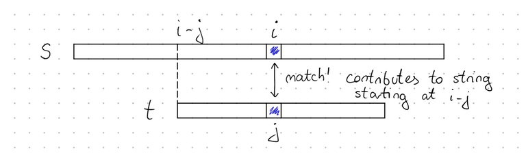
That is, the number of matching "a"-s in the string $$$s[k \ldots k + m - 1]$$$ is
$$$ \displaystyle \sum_{i - j = k} s_a [i] \cdot t_a [j]. $$$We must calculate this for all $$$k$$$ and have already learned how to efficiently calculate sums of this type.
Subset sum variations
Suppose you have $$$n$$$ rocks and the $$$i$$$-th of them weighs $$$a_i$$$ grams. How many ways are there to pick rocks such that their total weight is exactly $$$k$$$? Depending on the constraints and the exact problem, there are many ways to think about this. But one way is to model them is with polynomials. The answer to the question is exactly the coefficient of $$$x^k$$$ in the polynomial
$$$ (1 + x^{a_0}) (1 + x^{a_1}) (1 + x^{a_2}) \cdots (1 + x^{a_{n - 1}}). $$$Here is one problem where a similar perspective is useful.
Problem. (1096G - Lucky Tickets) We consider decimal numbers with even length $$$n$$$, potentially with leading zeroes. You are given a subset of decimal digits that are allowed. Count, modulo 998244353, the number of numbers with length $$$n$$$ that consist of only allowed digits and whose first $$$n / 2$$$ digits sum to the same value as the last $$$n / 2$$$ digits. $$$n \le 2 \cdot 10^5$$$.
SolutionLet $$$p(x) = p_0 x^0 + p_1 x^1 + \cdots + p_9 x^9$$$ where $$$p_d = 1$$$ if $$$d$$$ is allowed and $$$0$$$ otherwise. The number of ways to make $$$n / 2$$$ digits sum to $$$k$$$ is the coefficient of $$$x^k$$$ in $$$(p (x))^{n / 2}$$$. The polynomial $$$(p (x))^{n / 2}$$$ can be calculated by using FFT and fast exponentiation.
Thank you for reading! Please let me know how you liked it. I'm especially curious to hear what people think about hand-drawn figures.


Awesome work. Thanks for this gift.
I'm curious, how did you make the drawings?
I use a graphics tablet and a program called Xournal++.
-is-this-fft-
Omg, I literally made a post about need for a good FFT tutorial just a few minutes ago.
how do you transform a set of points to a polynomial
Nice tutorial!
Although, I would like to point out some moments which are kinda strange to me. These are very minor and don't influence the tutorial correctness, but nevertheless:
For applications, I would also add bignum multiplication, this is usually one of the most well-known instances of stating a problem in terms of polynomials.
Thank you, I have fixed these.
So the answer to the question -is-this-fft- is yes?
And now new question is: -is-this-fft- worth $300 ? xD
finally a fft blog by is-this-fft
Epic title drop
I tried finding in the past but couldn't find a source that illlustrates how to compute NTT modulo an arbitrary prime like $$$10^9+7$$$ using Chinese Remainder Theorem. Could you add a section describing that.
try this
- compute NTT modulo
998244353X = x1 mod 998244353- compute NTT modulo
7340033X = x2 mod 7340033use chinese remainder theorem to find a solution to X (there may be multiple solutions )
then do X mod(1e9 + 7)
NOTE: this works only when X <= 998244353 * 7340033, i.e., the final value shouldn't exceed 1e16. So this enumerates the rest of all solutions and only one solution exists.
Oh wow, that's awesome. Thanks a lot!
Lol, still 11
Cool!
Also, another way to compute inverse FFT is literally do the same operations as in the usual FFT, but inverse each of them and their order. That is, if your FFT looks like this:
then your inverse FFT may look like this:
This requires no thinking, and, in particular, doesn't involve the (beautiful) fact about the self-duality of FFT
I wonder if there is any way to calculate the inversion count of an array with FFT. Of course, we can use merge sort but still...
nice one! Thanks -is-this-fft-!
sorry for disturbing the comments after a while it has been posted but i have to sincerely thank for this gold.
2⋅p[x]<p[x]I think this should be corrected as2⋅p[x]<p[y]in the CSA problem of cross-correlationminor comment, 998244353 equal 2^23⋅7⋅17+1, not 2^23⋅7⋅11+1
I think there are some small typos.
"Let's reorder the columns of this matrix by bringing the even-numbered columns to the left and the odd-numbered columns to the left.". I think it should be bringing the odd-numbered columns to the right.
"Each query consists of two integers 1≤x<y≤n. For each query, calculate modulo 998244353 the number of permutations p of length n such that p[y]=maxyi=1p[i] and 2⋅p[x]<p[x]." I think the statement says 2.p[x] < p[y].
Because of this blog, I have finally been able to learn FFT, a concept that I believed to be above my reach. I am forever in your debt.
Thanks sir , i learnt fft from this tutorial. left is to solve questions linked.