


Hello, Codeforces!
At some point of life you want to make a new data structure problem with short statement and genius solution. LIS (Longest Increasing Subsequence) is a classic problem with beautiful solution, so you come up with the following problem:
- Given a sequence $$$A$$$ of length $$$N$$$ and $$$Q$$$ queries $$$1 \le i \le j \le N$$$, compute the length of Longest Increasing Subsequence of $$$A[i], A[i + 1], \ldots, A[j]$$$.
But on the other hand this looks impossible to solve, and you just give up the idea.
I always thought that the above problem is unsolved (and might be impossible), but very recently I learned that such queries are solvable in only $$$O(N \log^2 N + Q \log N)$$$ time, not involving any sqrts! The original paper describes this technique as semi-local string comparison. The paper is incredibly long and uses tons of scary math terminology, but I think I found a relatively easier way to describe this technique, which I will show in this article.
Thanks to qwerasdfzxcl for helpful discussions, peltorator for giving me the motivation, and yosupo and noshi91 for preparing this problem.
Chapter 1. The All-Pair LCS Algorithm
Our starting point is to consider the generalization of above problem. Consider the following problem:
- Given a sequence $$$S$$$ of length $$$N$$$, $$$T$$$ of length $$$M$$$, and $$$Q$$$ queries $$$1 \le i \le j \le M$$$, compute the length of Longest Common Subsequence of $$$S$$$ and $$$T[i], T[i + 1], \ldots, T[j]$$$.
Indeed, this is the generalization of the range LIS problem. By using coordinate compression on the pair $$$(A[i], -i)$$$, we can assume the sequence $$$A$$$ to be a permutation of length $$$N$$$. The LIS of the permutation $$$A$$$ is equivalent to the LCS of $$$A$$$ and sequence $$$[1, 2, \ldots, N]$$$. Hence, if we initialize with $$$S = [1, 2, \ldots, N], T = A$$$, we obtain a data structure for LIS query.
The All-Pair LCS problem can be a problem of independent interest. For example, it has already appeared in an old Petrozavodsk contest, and there is a various solution solving the problem in $$$O(N^2 + Q)$$$ time complexity (assuming $$$N =M$$$). Personally, I solved this problem by modifying the Cyclic LCS algorithm by Andy Nguyen. However, there is one particular solution which can be improved to a near-linear Range LIS solution, which is from the paper An all-substrings common subsequence algorithm.
Consider the DP table used in the standard solution of LCS problem. The states and transition form a directed acyclic graph (DAG), and have a shape of a grid graph. Explicitly, the graph consists of:
- $$$(N+1) \times (M+1)$$$ vertices corresponding to states $$$(i, j)$$$
- Edge of weight $$$0$$$ from $$$(i, j)$$$ to $$$(i+1, j)$$$ and $$$(i, j+1)$$$
- Edge of weight $$$1$$$ from $$$(i, j)$$$ to $$$(i+1, j+1)$$$ if $$$S[i+1] = T[j+1]$$$.
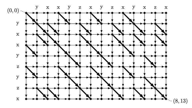
Figure: DAG constructed from the string "yxxyzyzx", "yxxyzxyzxyxzx"
Here, you can observe that the answer to the query $$$(i, j)$$$ corresponds to the longest path from $$$(0, i-1)$$$ to $$$(N, j)$$$. Let's denote the length of longest path from $$$(x_1, y_1)$$$ to $$$(x_2, y_2)$$$ as $$$dist((x_1, y_1), (x_2, y_2))$$$. Our goal is to compute $$$dist((0, i), (N, j))$$$ for all $$$0 \le i < j \le M$$$.
How can we do this? We need several lemmas:
Lemma 1. $$$dist((0, y), (i, j)) - dist((0, y), (i, j-1))$$$ is either $$$0$$$ or $$$1$$$.
Proof.
- $$$dist((0, y), (i, j-1)) \le dist((0, y), (i,j))$$$ since otherwise we can extend the path to $$$(i, j-1)$$$ with rightward edges.
- $$$dist((0, y), (i, j-1)) \geq dist((0, y), (i, j)) - 1$$$ since we can cut the path to $$$(i, j)$$$ exactly at the column $$$j - 1$$$ and move downward. $$$\blacksquare$$$
Lemma 2. $$$dist((0, y), (i, j)) - dist((0,y ), (i-1, j))$$$ is either $$$0$$$ or $$$1$$$.
Proof. Identical with Lemma 1. $$$\blacksquare$$$
Lemma 3. For every $$$i, j$$$, there exists some integer $$$0 \le i_h(i, j) \le j$$$ such that
- $$$dist((0, y), (i, j)) - dist((0, y), (i, j-1)) = 1$$$ for all $$$i_h(i, j) \le y < j$$$
- $$$dist((0, y), (i, j)) - dist((0, y), (i, j-1)) = 0$$$ for all $$$0 \le y < i_h(i, j)$$$
Proof. Above statement is equivalent of following: For all $$$y, i, j$$$ we have $$$dist((0, y), (i, j)) - dist((0, y), (i, j-1)) \le dist((0, y+1), (i, j)) - dist((0, y+1), (i, j-1))$$$. Consider two optimal paths from $$$(0, y) \rightarrow (i, j)$$$ and $$$(0, y+1) \rightarrow (i, j-1)$$$. Since the DAG is planar, two paths always intersect. By swapping the destination in the intersection, we obtain two paths $$$(0, y) \rightarrow (i, j-1)$$$ and $$$(0, y + 1) \rightarrow (i, j)$$$ which can not be better than optimal. Therefore we have $$$dist((0, y), (i, j)) + dist((0, y+1), (i, j-1)) \le dist((0, y+1), (i, j)) + dist((0, y), (i, j-1))$$$ which is exactly what we want to prove. $$$\blacksquare$$$
Lemma 4. For every $$$i, j$$$, there exists some integer $$$0 \le i_v(i, j) \le j$$$ such that
- $$$dist((0, y), (i, j)) - dist((0, y), (i-1, j)) = 0$$$ for all $$$i_v(i, j) \le y < j$$$
- $$$dist((0, y), (i, j)) - dist((0, y), (i-1, j)) = 1$$$ for all $$$0 \le y < i_v(i, j)$$$
Proof. Identical with Lemma 3. $$$\blacksquare$$$
Suppose we have the answer $$$i_h(i, j)$$$ and $$$i_v(i, j)$$$ for all $$$i, j$$$. How can we compute the value $$$dist((0, i), (N, j))$$$? Let's write it down:
$$$dist((0, i), (N, j)) \newline = dist((0, i), (N, i)) + \sum_{k = i+1}^{j} dist((0, i), (N, k)) - dist((0, i), (N, k-1)) \newline = 0 + \sum_{k = i+1}^{j} (i_h(N, k) <= i)$$$
It turns out that we don't even need all values, we only have to know a single linear array $$$i_h(N, *)$$$ ! Given that we have an array $$$i_h(N, *)$$$, the queries can be easily answered in $$$O(\log N)$$$ time with Fenwick trees, or $$$O(1)$$$ time if we use $$$N^2$$$ precomputation.
Hence, all we need to do is to compute the values $$$i_h$$$ and $$$i_v$$$, and it turns out there is a very simple recurrence.
Theorem 5. The following holds:
- $$$i_h(0, j) = j$$$
- $$$i_v(i, 0) = 0$$$
- For $$$i, j \geq 1$$$ and $$$S[i] = T[j]$$$
- $$$i_h(i, j) = i_v(i, j-1)$$$
- $$$i_v(i, j) = i_h(i-1, j)$$$
- For $$$i, j \geq 1$$$ and $$$S[i] \neq T[j]$$$
- $$$i_h(i, j) = \max(i_h(i-1, j), i_v(i, j-1))$$$
- $$$i_v(i, j) = \min(i_h(i-1, j), i_v(i, j-1))$$$
Proof. Base cases are trivial. For a fixed $$$y$$$, consider the distance from $$$(0, y)$$$ to the four cells in the rectangle $$$(i-1, j-1), (i-1, j), (i, j-1)$$$. Let $$$t = dist((0, y), (i-1, j-1))$$$, then the other two cells either attain value $$$t$$$ or $$$t + 1$$$. Therefore, the possibilities are:
- $$$dist((0, y), (i-1, j))$$$ having value $$$t$$$ or $$$t + 1$$$ (equivalently, $$$y \ge i_h(i - 1, j)$$$)
- $$$dist((0, y), (i, j-1))$$$ having value $$$t$$$ or $$$t + 1$$$ (equivalently, $$$y < i_v(i, j-1)$$$)
- Whether $$$S[i] = T[j]$$$ or not
Those three values uniquely determine $$$dist((0, y), (i, j))$$$. You can verify the Theorem 5 by manually inspecting all $$$2^3 = 8$$$ cases by hand. $$$\blacksquare$$$
Remark. At least this is the proof I found, and this is also the proof from the original paper. I believe there is a simpler interpretation, so please add a comment if you have a good idea!
As Theorem 5 gives a simple recurrence to compute all values $$$i_h$$$ and $$$i_v$$$, we can solve the All-Pair LCS problem in $$$O(NM + Q \log N)$$$ time, hence the Range LIS problem in $$$O(N^2 + Q \log N)$$$ time.
As long as SETH Conjecture is true, the longest common subsequence of two strings can not be computed faster than $$$O(NM)$$$ time. Hence our algorithm has no room for improvement. However, in the case of LIS, one of our pattern is fixed as $$$[1, 2, \ldots, N]$$$, and it turns out we can use this to improve the time complexity.
Chapter 2. The Seaweed
Visualizing the above DP procedure gives a further insight on the structure. We can consider the value $$$i_v$$$ and $$$i_h$$$ to be associated with the edges of the grid: In that sense, the DP transition is about picking the values from the upper/left edges, and routing them to the lower/right edges of the rectangular cell. For example, we can draw a following picture: 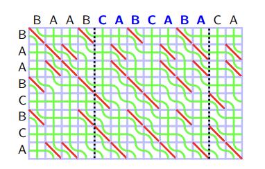
In this picture, green curves represent the values — values from the left edges of big rectangle ("BAABCBCA") are $$$0$$$, from the upper edges of big rectangle ("BAABCABCABA") are $$$1, 2, \ldots, M$$$. We will call each green curve as a seaweed. We will also read the seaweed from the lower left corner to the upper right corner, and say the seaweed is in left or right according to this order. In this regard, in the beginning seaweeds are sorted in the increasing order.
Let's reinterpret the DP transition from Theorem 5 with this visualization. If $$$S[i] = T[j]$$$, two seaweed do not intersect. If $$$S[i] \neq T[j]$$$, two seaweed intersect if the right seaweed have a greater value than the left one. In other words, each cell $$$S[i] \neq T[j]$$$ is the anti-sorter of seaweed: If two adjacent seaweeds $$$i, i+1$$$ have increasing values ($$$A[i] < A[i +1]$$$), it swaps so that they have decreasing values ($$$A[i] > A[i+1]$$$).
Of course, in the case of Range LIS we have $$$N^2 - N$$$ such pair, so this is still not enough to solve the problem, but now I can present a main idea for optimization.
Suppose that we swap two values regardless of their values. We can represent each operation as a permutation $$$P$$$ where $$$P(i)$$$ stores the final position of $$$i$$$-th seaweed from the beginning. Let's say we have a swap operation in position $$$i_1, i_2, \ldots, i_k$$$, and let the elementary permutation $$$P_i$$$ be
$$$\begin{equation}P_i(j)=\begin{cases} j+1, & \text{if}\ a=i \newline j-1, & \text{if}\ a=i+1 \newline j, & \text{otherwise}\end{cases} \end{equation}$$$
Then the total operation can be described as a single permutation $$$P = P_{i_1} \circ P_{i_{2}} \circ \ldots \circ P_{i_k}$$$ where $$$P \circ Q$$$ is a composite permutation: $$$P \circ Q(i) = Q(P(i))$$$.
We can't use this to solve the Range LIS problem because we take the values into account. But very surprisingly, even with that condition, there exists a cool operator $$$\boxdot$$$ such that:
- $$$\boxdot$$$ is associative.
- The total operation can be described as a single permutation $$$P = P_{i_1} \boxdot P_{i_{2}} \boxdot \ldots \boxdot P_{i_k}$$$
Chapter 3. The Operator
The definition of this operator is pretty unintuitive, and needs several auxiliary lemmas:
Definition 6. Given a permutation $$$P$$$ of length $$$N$$$, let $$$\Sigma(P)$$$ be the $$$(N+1) \times (N+1)$$$ square matrix, such that $$$\Sigma(P)_{i, j} = |\{x|x \geq i, P[x] < j\}|$$$
Intuitively, it is a partial sum in left-down direction, for example, if $$$P = [2, 3, 1]$$$, we have:
$$$\Sigma(P) = \begin{bmatrix} 0&1&2&3 \newline 0&1&1&2 \newline 0&1&1&1 \newline 0&0&0&0 \end{bmatrix}$$$
Which is the partial sum of $$$\begin{bmatrix} 0&0&1&0 \newline 0&0&0&1 \newline 0&1&0&0\newline 0&0&0&0 \end{bmatrix}$$$.
Definition 7. Given two matrix $$$A$$$ of size $$$N \times M$$$, $$$B$$$ of size $$$M \times K$$$, the min-plus multiplication $$$A \odot B$$$ is $$$(A \odot B)_{i, j} = min_{1 \le k \le M} (A_{i, k} + B_{k, j})$$$.
Theorem 8. Given two permutation $$$P, Q$$$ of length $$$N$$$, there exists a permutation $$$R$$$ of length $$$N$$$ such that $$$\Sigma(R) = \Sigma(P) \odot \Sigma(Q)$$$. We denote such $$$R$$$ as $$$P \boxdot Q$$$.
To prove it we need two lemmas:
Lemma 8.1. For a matrix $$$\Sigma(R)$$$, there exists a permutation $$$R$$$ if and only if the following conditions are satisfied:
- $$$\Sigma(R)_{i, 1} = 0$$$
- $$$\Sigma(R)_{N+1, i} = 0$$$
- $$$\Sigma(R)_{i, N+1} = N + 1 - i$$$
- $$$\Sigma(R)_{1, i} = i - 1$$$
- $$$\Sigma(R)_{i, j} - \Sigma(R)_{i, j-1} - \Sigma(R)_{i+1, j} + \Sigma(R)_{i+1, j-1} \geq 0$$$
Proof of Lemma 8.1. Consider the inverse operation of partial sums. We can always restore the permutation if the "inverse partial sum" of each row and column contains exactly one $$$1$$$ for each rows and columns, and $$$0$$$ for all other entries. Fifth term guarantees that the elements are nonnegative, third and fourth term guarantees that each rows and columns sums to $$$1$$$. Those conditions are sufficient to guarantee that the inverse yields a permutation. $$$\blacksquare$$$
Lemma 8.2. For any matrix $$$A$$$, $$$A_{i, j} - A_{i, j-1} - A_{i+1, j} + A_{i+1, j-1} \geq 0$$$ for all $$$i, j$$$ if and only if $$$A_{i_1, j_2} - A_{i_1, j_1} - A_{i_2, j_2} + A_{i_2, j_1} \geq 0$$$ for all $$$i_1 \le i_2, j_1 \le j_2$$$.
Proof of Lemma 8.2. $$$\rightarrow$$$ is done by induction. $$$\leftarrow$$$ is trivial. $$$\blacksquare$$$
Proof of Theorem 8. We will prove the first four points of Lemma 9. Note that all entries of $$$\Sigma(R)$$$ are nonnegative since $$$\Sigma(P), \Sigma(Q)$$$ does.
- $$$\Sigma(R)_{i, 1} \le \Sigma(P)_{i, 1} + \Sigma(Q)_{1, 1} = 0$$$
- $$$\Sigma(R)_{N+1, i} \le \Sigma(P)_{N+1, N+1} + \Sigma(Q)_{N+1, i} = 0$$$
- $$$\Sigma(R)_{i, N + 1} = \min(\Sigma(P)_{i, j} + \Sigma(Q)_{j, N+1}) = \min(\Sigma(P)_{i, j} + N+1-j)$$$. Considering the derivative, the term is minimized when $$$j = N + 1$$$. $$$\Sigma(R)_{i, N+1} = \Sigma(P)_{i, N+1} = N+1-i$$$
- $$$\Sigma(R)_{1, i} = \min(\Sigma(P)_{1, j} + \Sigma(Q)_{j, i}) = \min(j-1 + \Sigma(Q)_{j, i})$$$. Considering the derivative, the term is minimized when $$$j = 1$$$. $$$\Sigma(R)_{1, i} = \Sigma(Q)_{1, i} = i-1$$$
Here, when we consider the derivative, we use the fact that $$$0 \le \Sigma(P)_{i, j} - \Sigma(P)_{i, j - 1} \le 1$$$. $$$N + 1 - j$$$ definitely decreases by $$$1$$$ when we increase the $$$j$$$, but $$$\Sigma(P)_{i, j}$$$ never increases more than $$$1$$$ even when we increase the $$$j$$$. Therefore, it does not hurt to increase the $$$j$$$. We will use this technique later on.
To prove the final point, let $$$k_1, k_2$$$ be the index where $$$\Sigma(R)_{i, j} = \Sigma(P)_{i, k_1} + \Sigma(Q)_{k_1, j}$$$, $$$\Sigma(R)_{i+1, j-1} = \Sigma(P)_{i+1, k_2} + \Sigma(Q)_{k_2, j-1}$$$. Suppose $$$k_1 \le k_2$$$, we have
$$$\Sigma(R)_{i, j-1} + \Sigma(R)_{i+1, j} \newline = \min_k (\Sigma(P)_{i, k} + \Sigma(Q)_{k, j-1}) + \min_k (\Sigma(P)_{i+1, k} + \Sigma(Q)_{k, j}) \newline \le \Sigma(P)_{i, k_1} + \Sigma(P)_{i+1, k_2} + \Sigma(Q)_{k_1, j-1} + \Sigma(Q)_{k_2, j} \newline \le \Sigma(P)_{i, k_1} + \Sigma(P)_{i+1, k_2} + \Sigma(Q)_{k_1, j} + \Sigma(Q)_{k_2, j-1} \newline =\Sigma(R)_{i, j} + \Sigma(R)_{i+1, j-1}$$$
(Note that Lemma 8.2 is used in $$$\Sigma(Q)$$$)
In the case of $$$k_1 \geq k_2$$$ we proceed identically, this time using the Lemma 8.2 for $$$\Sigma(P)$$$. $$$\blacksquare$$$
Theorem 9. The operator $$$\boxdot$$$ is associative.
Proof. Min-plus matrix multiplication is associative just like normal matrix multiplication. $$$\blacksquare$$$
Lemma 10. Let $$$I$$$ be the identity permutation ($$$I(i) = i$$$), we have $$$P \boxdot I = P$$$ (For proof you can consider the derivative.) $$$\blacksquare$$$
And now here comes the final theorem which shows the equivalence of the "Seaweed" and the "Operator":
Theorem 11. Consider the sequence of $$$N$$$ seaweed and sequence of operation $$$i_1, i_2, \ldots, i_k$$$, where each operation denotes the following:
- In the beginning, there is $$$i$$$-th seaweed in $$$i$$$-th position.
- For each $$$1 \le x \le k$$$, we swap the seaweed in $$$i_x$$$ th position and $$$i_x + 1$$$ th position, only if the seaweed $$$i_x$$$ has smaller index than seaweed $$$i_x+1$$$.
Let $$$P_i$$$ be the elementary permutation as defined above. Let $$$P = P_{i_1} \boxdot P_{i_{2}} \boxdot \ldots \boxdot P_{i_k}$$$ . Then after the end of all operation, $$$i$$$-th seaweed is in the $$$P(i)$$$-th position.
Proof of Theorem 11. We will use induction over $$$k$$$. By induction hypothesis $$$P_{i_1} \boxdot P_{i_{2}} \boxdot \ldots \boxdot P_{i_{k-1}}$$$ correctly denotes the position of seaweeds after $$$k - 1$$$ operations. Let
- $$$t = i_k$$$
- $$$A = P_{i_1} \boxdot P_{i_{2}} \boxdot \ldots \boxdot P_{i_{k-1}}$$$
- $$$B = P_{i_1} \boxdot P_{i_{2}} \boxdot \ldots \boxdot P_{i_{k}}$$$
- $$$A(k_0) = t, A(k_1) = t+1$$$
It suffices to prove that
- $$$B(k_0) = t+1, B(k_1) = t, B(i) = A(i)$$$ for all other $$$i$$$ if $$$k_0 < k_1$$$
- $$$B= A$$$ if $$$k_0 > k_1$$$
Which is also equivalent to:
- $$$\Sigma(B)_{i, j} = \Sigma(A)_{i, j} + 1$$$ if $$$k_0 < i \le k_1, j = t + 1$$$
- $$$\Sigma(B)_{i, j} = \Sigma(A)_{i, j}$$$ otherwise.
Observe that $$$\Sigma(P_t) - \Sigma(I)$$$ has only one nonzero entry $$$(\Sigma(P_t) - \Sigma(I))_{t+1, t+1} = 1$$$. Since we know $$$\Sigma(A) \odot \Sigma(I) = \Sigma(A)$$$, $$$\Sigma(B)$$$ and $$$\Sigma(A)$$$ only differs in the $$$t+1$$$-th column. For the $$$t + 1$$$-th column, note that
$$$\Sigma(B)_{i, t + 1}$$$ $$$= \min_j (\Sigma(A)_{i, j} + \Sigma(P_t)_{j, t + 1})$$$ $$$= \min(\min_{j \le t} (\Sigma(A)_{i, j} + t + 1 - j), \Sigma(A)_{i, t + 1} + 1, (\min_{j > t+1} \Sigma(A)_{i, j})$$$ $$$= \min(\Sigma(A)_{i, t} + 1,\Sigma(A)_{i, t + 2})$$$ (derivative)
If $$$k_0 < k_1$$$, we have
- $$$\Sigma(A)_{i, t} = \Sigma(A)_{i, t + 1} - 1 = \Sigma(A)_{i, t + 2} - 2$$$ ($$$i \le k_0$$$)
- $$$\Sigma(A)_{i, t} = \Sigma(A)_{i, t + 1} - 0 = \Sigma(A)_{i, t + 2} - 1$$$ ($$$k_0 < i \le k_1$$$)
- $$$\Sigma(A)_{i, t} = \Sigma(A)_{i, t + 1} - 0 = \Sigma(A)_{i, t + 2} - 0$$$ ($$$k_1 < i$$$)
Which you can verify $$$\Sigma(B)_{i, t+1} = \Sigma(A)_{i, t+1} + 1$$$ iff $$$k_0 < i \le k_1$$$
If $$$k_0 > k_1$$$, we have
- $$$\Sigma(A)_{i, t} = \Sigma(A)_{i, t + 1} - 1 = \Sigma(A)_{i, t + 2} - 2$$$ ($$$i \le k_1$$$)
- $$$\Sigma(A)_{i, t} = \Sigma(A)_{i, t + 1} - 1 = \Sigma(A)_{i, t + 2} - 1$$$ ($$$k_1 < i \le k_0$$$)
- $$$\Sigma(A)_{i, t} = \Sigma(A)_{i, t + 1} - 0 = \Sigma(A)_{i, t + 2} - 0$$$ ($$$k_0 < i$$$)
Which you can verify $$$\Sigma(B)_{i, t+1} = \Sigma(A)_{i, t+1}$$$ $$$\blacksquare$$$
Yes, this is a complete magic :) If anyone have good intuition for this result, please let me know in comments. (The original paper mention some group theory stuffs, but I have literally zero knowledge on group theory, and I'm also skeptical on how it helps giving intuition)
What's next
We learned all the basic theories to tackle the problem, and obtained an algorithm for the Range LIS problem. Using all the facts, we can:
- Implement the $$$\boxdot$$$ operator in $$$O(N^3)$$$ time
- Use the $$$\boxdot$$$ operator for $$$O(N^2)$$$ time
Hence we have... $$$O(N^5 + Q \log N)$$$ time algorithm. Of course this is very slow, but in the next article we will show how to optimize this algorithm to $$$O(N \log^2 N + Q \log N)$$$. We will also briefly discuss the application of this technique.
Practice problem
- Yosupo Judge: Prefix-Substring LCS
- BOJ: LCS 9
- IZhO 2013: Round words
- Ptz Summer 2019 Day 8: Square Subsequences


Hello. In blog, you say:
Isn't the longest path always like the manhattan distance (because you only go horisontally or vertically)? Why isn't it like difference between mahattan distance and shortest path (because it is like how many diagonal edges there are which iirc is what is counted in LCS code)?
In the DAG horizontal/vertical edges have weight $$$0$$$.
In Korean competitive programming communities, those ⊡ operators are called "nemo-jjijji" (square tits).
That's so qwerasdfzxcl-ish
Who disliked that comment will have gf with square tits :D
Can I have girlfriend by disliking that comment? (With square tits, anyway)
Relationship between LIS and LCS. Amazing!
Wuhu! Unit monge-matrix,it will become another well-known technology in china and I want to present such a problem in UOJ.
Amazing blog! A new technique for Div1D-E-F or OI problems, isn't it?
the DP in Chapter 1 gives a way to calculate the length of the LIS. Is it possible to calculate an example of some LIS from this DP?
length of LIS is given by number of indexes k where k in [i+1,j] and h(N,k)<=i; so I thought maybe an example of some LIS is the set of indexes k where k in [i+1,j] and h(N,k)<=i; but it's wrong
Thank you for nice blog!
(1) Explanation using the "longest path" interpretation.
I believe this proof is relatively straightforward, but it might not differ significantly from the "2^3-case by hand" proof.
Let $$$Y(0,y), A(i-1,j-1), B(i-1,j), C(i,j-1), D(i,j)$$$. If $$$S[i]=T[j]$$$, there exists a longest path from $$$Y$$$ to $$$D$$$ which use the diagonal edge $$$AD$$$, so we have $$$YD=YA+1$$$. Therefore, $$$y\geq i_h(i,j) \iff YD = YC+1 \iff YA=YC\iff y\geq i_v(i,j-1)$$$, and this proves the formula for $$$i_h(i,j)$$$. The formula for $$$i_v(i,j)$$$ is similar.
Next, assume $$$S_i\neq T_j$$$. In this case, $$$YD=\max(YB,YC)$$$. So $$$YD = YC+1 \iff YB=YC+1 \iff (YB,YC) = (YA+1,YA)$$$. This means $$$y\geq i_h(i,j) \iff y\geq \max(i_h(i-1,j),i_w(i,j-1)$$$ and the formula for $$$i_h(i,j)$$$ is proved.
(2) Explanation using the "LCS" interpretation.
I denote substring $$$S_l\cdots S_r$$$ by $$$S[l:r]$$$. Because $$$dist((0,y),(i,j)) = LCS(S[1:i], T[y:j])$$$, we can interpret the difference of dist as follows.
I think that even if we think this interpretation, we need some discussion which is essentially same as the "longest-path" discussion. But I think that we can understand the meaning of the formula more easily.
In case of $$$S[i] = T[j]$$$, consider four statements.
Then the formula of $$$i_h(i,j)$$$ correspond to the equivalence $$$1\iff 2$$$. Also the formula of $$$i_v(i,j)$$$ correspond to the equivalence $$$3\iff 4$$$.
In case of $$$S[i] \neq T[j]$$$.
Then, the formula of $$$i_h(i,j)$$$ correspond to $$$1 \iff 2\land 3$$$.