


While looking up an editorial for a CSES task, I recently stumbled upon CSES DP Section editorial blog by icecuber. Noticing that a few new tasks had been added since the blog was posted 2 years back; I decided to take his permission and write this blog, which contains editorials to the newly added tasks and acts as a sequel to his blog.
I would like to thank dominique38 for being the most enthusiastic co-author possible, defnotmee for being the second most enthusiastic co-author (he wanted the title himself), Perpetually_Purple for helping me out and giving suggestions, AntennaeVY for suggestions on the understandability and formatting of the blog; and finally, icecuber himself for going over the blog and giving me confidence in the form of a final thumbs-up!
The editorials may at some point appear excessively lengthy, but that is intended. Since CSES tasks are meant to teach standard approaches and techniques; I wanted this blog to be able to act as a substantially self-sufficient resource to learn the involved technique instead of just telling what technique to use to arrive at the solution and giving the implementation in code.
I would urge readers to first try to solve the problems themselves; and only then refer to the editorials. This will maintain the purpose and spirit of the CSES Problem Set.
All the problems are from the CSES Problemset.
Counting Towers (2413)
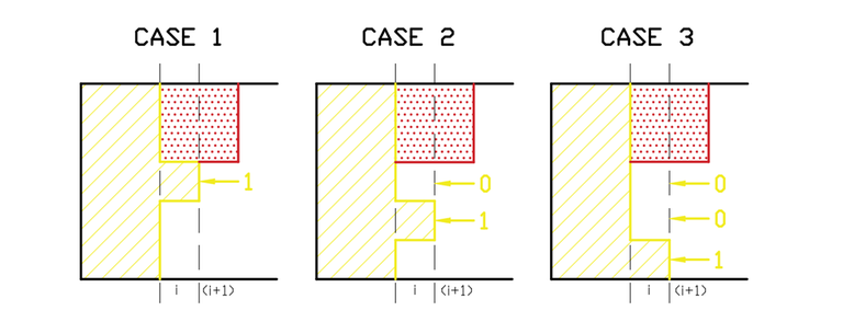
We define our dp state as dp[h] = the number of possible towers of height h. We now look at the possible solutions for towers of heights 1 and 2 to understand how to transition between the states of our dynamic programming.

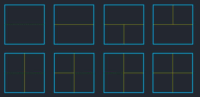
Here we can observe the following -
If we have a block of width 2 at the top of the tower of height $$$(n - 1)$$$; we have two ways to create a tower of height $$$n$$$ which has a block of width 2 at the top, either by increasing the height of the block on position $$$(n - 1)$$$ by $$$1$$$ or creating a new block of width 2 on position $$$n$$$ (as illustrated by the first two solutions on $$$n = 2$$$). Moreover, if we have a tower of height $$$(n - 1)$$$ with two blocks of width 1 on top we can only make a tower of height $$$n$$$ with a block of width 2 on the top by creating a new block of width 2 (third solution on $$$n = 2$$$)
If we have two blocks of width 1 at the top of the tower of height $$$(n - 1)$$$; we have four ways to create a tower of height $$$n$$$ which has two blocks of width 1 at the top (solutions 5, 6, 7 and 8). This is because we have the option to increase the height of one of the pre-existing blocks or place a new block of width 1 above a pre-existing block. This gives us the four options as shown in the illustration. Moreover, we can have a tower of height $$$n$$$ with two blocks of width 1 at the top if we have a tower of height $$$(n - 1)$$$ with a block of width 2 at the top by creating two new blocks of width 1 (solution 4).
We are only concerned about the changes happening at the top of the existing tower. This is because we can only add blocks or increase the height of existing blocks at the top of the towers, which is only dependent on what was on top of the tower before. That way, we can find the answer for any $$$n$$$ if we consider that all the subproblems for towers of smaller heights have already been solved since we construct our dp table in a bottom-up manner.
Note: Green dashed lines in the images mean that we replaced a block of height $$$h$$$ with a block of height $$$(h + 1)$$$ at the top of the tower.
The total number of possible ways to have a tower of height $$$n$$$ will be the sum of the number of towers with two blocks of width 1 at the top and the towers with a block of width 2 at the top. Using the observations above we can build our transitions.
Overall Time Complexity: $$$O(1e6)$$$ for pre-computation; and $$$O(t)$$$ for the test cases.
Link to Code in CPP $$$\cdot$$$ Link to Code in Python
Projects (1140)
This task is based on the well-known Interval Scheduling Problem. If interested, it's worth checking out this lecture on MIT OCW which discusses this problem. More specifically, this task is based on the Weighted Interval Scheduling variation. In this, we need to schedule the subset of requests of maximal weight that are non-overlapping, where each request $$$i$$$ has weight $$$w(i)$$$. A key observation here is that the greedy algorithm no longer works, since just taking the element with the lowest $$$r_i$$$ may prevent you from choosing an element with high weight.
Let us first go over the naive approach. To solve this problem, we need to find the optimal $$$r_{j}$$$ (end-scheduling-time) that gives maximum overall value for given $$$i$$$, when we add the task at $$$a[i]$$$. We sort the tasks by $$$r_i$$$ and define our dp state as dp[i] = maximum weight of an optimal subset whose last task is the task i. For this, we will go over every possible $$$j$$$ such that that $$$r_{j} < l_{i}$$$ (ending time of $$$a[j]$$$ less than the starting time of $$$a[i]$$$). We will have a $$$O(n)$$$ transitions per state, which are given as $$$dp[i] = w(i) + max_{r_{j}<l_{i}}(dp[j])$$$, totaling a complexity of $$$O(n^2)$$$
The quadratic order arises because we don't know where the optimal $$$r_{j}$$$ lies. However, if we have that information, we can change the definition of our dp to dp[i] = maximum weight of an optimal subset considering only elements with end time less or equal to the end time of i. This idea is like maintaining a prefix-maximum of our original $$$dp[i]$$$ based on $$$r_{i}$$$. Once we have this, we can easily binary search for the closest non-overlapping $$$r_{j}$$$ to the left and take value $$$dp[j]$$$; which will give us the best value up to that point (since prefix-maximum is non-decreasing and going further left will give us worse values). In this approach, the transitions will become $$$dp[i] = max(w(i) + dp[j],dp[i-1])$$$.
In our task we can only do one project at a time; and we need to select a subset of non-overlapping projects that will reward us with the maximum money. Firstly, we sort the projects in ascending order of their ending dates. We now construct a dp array, where dp[i] = maximum money that we can have at the end of the ith end date. When we are on a project, we can either choose to take it or ignore it — and we need to take choose the option that allows us to get more money. If we choose to take the project at hand, we will need to add the project's reward to the money we have received from projects that end before the current project starts.
Time Complexity: $$$O(n \cdot \log{n})$$$
Link to Code in CPP $$$\cdot$$$ Link to Code in Python
Elevator Rides (1653)
This is a standard variation of the Knapsack problem, famously known as the bin-packing problem. It uses the idea of bitmask DP; so if you don't know that, then this Bitmask Dynamic Programming video by tehqin can be a great place to get started.
We are given that $$$n \leq 20 $$$ and since $$$2^{20} \approx 10^{6}$$$ we can use bitmasks as indices to store all possible states (that state being a subset of people we are considering); where the $$$i$$$th bit being set means that the $$$i$$$ th person is included in that subset. We now define our dp state as dp[X] = minimum number of rides needed for the subset X of people.
To find the best answer for $$$X$$$ let's try shuffling the weights to find the best possible configuration of weight distribution.
Naive Approach:
Let us select some subset $$$x$$$ of $$$X$$$ such that for every set bit at the $$$i$$$ th position in $$$x$$$ we have $$$\sum_{i}^{x} w(i) \leq S$$$, where $$$S$$$ is the maximum allowed weight in the elevator. If we fix that $$$x$$$ will be in the same elevator ride, we can update $$$dp[X]$$$ by making the transition:
Here we are choosing which subset $$$x$$$ is in the first elevator ride and saying that the required number of elevator rides will be 1 (the elevator ride of $$$x$$$) + the best configuration for the subset X - x (that is, $$$dp[X - x]$$$), which we already know since we construct the DP in bottom-up order.
Also note that since $$$x$$$ is a subset of $$$X$$$; X - x is the same as X ^ x (taking bitwise XOR) and can be used interchangeably. Bitwise operations can be considered to be a better choice since they are faster in practice than normal algebraic operations.
We also need to pre-calculate the sum of weights for each of the bitmasks (subsets) to avoid increasing the complexity while calculating $$$dp[X]$$$. The pseudo-code for this approach is given below:
Time Complexity of this approach: Let's think how many times a bitmask of $$$k$$$ set bits will get iterated by. There are $$$\binom{n}{k}$$$ such masks and they will get iterated $$$2^{n-k}$$$ times each. That way, the total number of iterations is $$$\sum_{k=0}^{n} \binom{n}{k}*2^{n-k} = (1+2)^{n} = 3^n$$$, totaling a $$$O(3^n)$$$ algorithm. A way to see why this is true is observing that the number of ways to make a number of $$$n$$$ digits in base $$$3$$$ with $$$k$$$ zeroes is $$$\binom{n}{k}*2^{n-k}$$$ (choosing which $$$k$$$ digits will be zero and choosing whether the $$$n-k$$$ remaining bits will be $$$1$$$ or $$$2$$$), so the sum of it for all $$$k$$$ will be the total amount of numbers of $$$n$$$ digits in base $$$3$$$, that is, $$$3^n$$$.
This $$$O(3^n)$$$ algorithm works for $$$ n \approx 16$$$ but not for $$$n=20$$$, so we need to come up with a better approach.
Optimization:
The approach above has 2 problems:
We are iterating over all $$$x \subseteq X$$$ which is bounded by $$$3^n$$$
Even between answers using the same subset and with the same number of elevator rides, some of them are better than others. For example, an answer where all the empty space is on exactly one of the elevator rides allows for more choice than an answer where there is exactly 1 empty space in each of the elevator rides.
To fix those problems, for a given set X let's try to fix which $$$i$$$ will be the last person we put in the last elevator ride of our optimal answer for that set. If we follow that definition and we have a given configuration of rides for the subset $$$(X - i)$$$ we can two things with $$$i$$$:
Put $$$i$$$ together with the last elevator ride used by the configuration of $$$(X - i)$$$.
Create a new elevator ride and put $$$i$$$ in it.
That way, the only attributes that matter for a configuration for the set $$$(X - i)$$$ is the number of elevator rides it uses (which we will call $$$k$$$) and the ammount of space already used in the last ride of that configuration (which we will call $$$W$$$). We would like to know for any 2 given configurations of elevator rides for the set $$$(X-i)$$$, which one would be optimal to create an answer for set $$$X$$$. Let's say those configurations are $$$c_1$$$ and $$$c_2$$$ with attributes $$$\lbrace k_1,W_1 \rbrace$$$ and $$$\lbrace k_2,W_2 \rbrace$$$ respectively, and analyze the possible cases.
- If $$$k_1 \leq k_2$$$ and $$$W_1 \leq W_2$$$, $$$c_1$$$ is obviously better than $$$c_2$$$
- If $$$k_1 < k_2$$$ but $$$W_1 > W_2$$$, $$$c_1$$$ is still better. The reason is that even if we are forced to create a new elevator ride because $$$w(i) + W_1 > S$$$, we will reach a configuration of attributes $$$\lbrace k_1+1,w(i) \rbrace$$$, which is clearly better than both configurations reachable from $$$c_2$$$: $$$\lbrace k_2, W+w(i) \rbrace$$$ and $$$\lbrace k_2+1, w(i) \rbrace$$$
That way, it is always optimal to minimize $$$k$$$ in a given configuration and, after that, minimize $$$W$$$.
Let's now define our dp state as $$$dp[X] = \lbrace k , W \rbrace $$$, where $$$k =$$$ minimum number of rides needed for $$$X$$$ (just like before) and $$$W = $$$ minimum weight on the last elevator ride given that $$$k$$$ is minimum. We will now add the person weights to our answer one at a time; instead of considering the weight of the entire submask like before. Note that it is often quite difficult to minimize 2 parameters simultaneously; but here we can safely make the transitions due to our observation. We will first minimize $$$k$$$, then we minimize $$$W$$$.
When we fix that $$$i$$$ is the last person in our subset, let's say we have $$$dp[X \oplus 2^i] = \lbrace k, W \rbrace$$$. We now have to check if adding the person to last elevator ride exceeds the maximum allowed weight in the elevator. If so, we increase the number of required rides by 1, and the weight of the new last rides becomes the weight of the person being added:
Else we can just add $$$i$$$ to the last elevator ride used by $$$dp[X \oplus 2^i]$$$:
We now analyze our improved time complexity. We don't have to iterate over subsets $$$x$$$ anymore. Instead, for each bitmask we just iterate over the elements in it one by one, leading to a final complexity of $$$O(n \cdot 2 ^ n)$$$, which will easily pass for $$$n \leq 20$$$.
Link to Code (in CPP) $$$\cdot$$$ Link to Code (in Python)
For a more detailed idea, I suggest reading this Article or watch this video on Knapsack problems by Pavel Mavrin (pashka).
Counting Tilings (2181)
Let us start by trying to fill up the given grid using our dominoes in some ordered manner. Let us start by trying to tile one column of the given grid at a time. Say, at some point of time, the given grid looks as shown below:
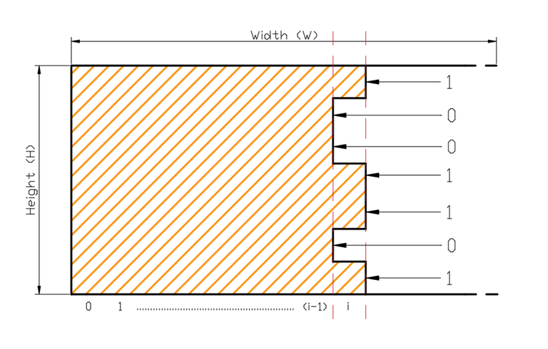
We are currently at the $$$i$$$th column which is not necessarily completely filled and all columns before that are filled with $$$2 \times 1$$$ and $$$1 \times 2$$$ tiles. We can see that some tiles are poking out into the $$$i$$$th column. These poking out tiles can only be from column $$$i-1$$$, which means we only need information about the previous column when we are tiling any given column. Now each of the $$$n$$$ cells in the column can either be tiled or be empty based on previous column; and hence we can use a bitmask to represent each of the possible states of the columns where a set bit in a bitmask means the corresponding cell of the column is tiled. The first thing to notice here is the constraints which are $$$n \leq 10 $$$ and $$$m \leq 1000 $$$. This suggests that we can use bitmasking only on rows. In order to build our solution; we take the $$$(n \times m)$$$ grid with n rows and m columns; and consider one column at a time. The size of each column being considered is now $$$n$$$.
We will now need to look at the number of ways we can arrive at a particular combination for a column. For example, if we place a $$$(1 \times 2)$$$ tile at a cell of one column, the cell of that corresponding row in the next column also gets tiled.
First Approach:
We are given current mask $$$X$$$ for the $$$i^{th}$$$ column which represents the cells already filled in it by poking tile pieces from the $$$(i-1)^{th}$$$ column. In the above diagram its $$$X = 1001101$$$. When we try to generate a new mask $$$X'$$$ for the $$$(i+1)^{th}$$$ column, there are multiple restrictions we have to follow. For example:
    X                X'
prev mask         mask now
    1     -->    only 0 is allowed, we can't put a horizontal tile on it
    0     -->    only 1 is allowed, we can't keep it empty and can't use a vertical tile
    1     -->       ~
    0     -->    1 and 0 are both allowed, we can place either 1 vertical tile or 2 horizontal tiles
    0
Let's try to understand what are the properties that make $$$X$$$ and $$$X'$$$ a valid transition:
If $$$X_j$$$ is the $$$j^{th}$$$ bit of $$$X$$$, it's impossible that both $$$X_j$$$ and $$$X'_j$$$ are active. That is because $$$X'_j$$$ is only active if we place a horizontal piece on the $$$j^{th}$$$ row of the $$$i^{th}$$$ column, which we can't do since $$$X_j$$$ is already active.
Consider the bits that are inactive in both $$$X$$$ and $$$X'$$$. The rows that fit that category are that way because we tiled the corresponding rows for those bits on column $$$i$$$ with vertical pieces. One of the ways to check if this is possible is seeing if every maximal segment of bits that are inactive in both $$$X$$$ and $$$X'$$$ has even size.
Note that if both conditions are satisfied, there is exactly one way to tile column $$$i$$$ with pieces to achieve given $$$X'$$$ from $$$X$$$, so they are necessary and sufficient to see if a transition is possible. From now on we will refer to that as the masks being compatible, and the conditions for it to happen are conditions $$$(1)$$$ and $$$(2)$$$ as above.
Now, let's define our dp state as $$$dp[i][X] =$$$ number of ways we can have the first $$$i$$$ columns completely filled (i.e., columns are completely filled until the $$$(i-1)^{th}$$$ column); such that mask $$$X$$$ is poking into the $$$i^{th}$$$ column. With this definition our final answer will be $$$dp[Width+1][0]$$$ (we will have filled columns $$$1$$$ through $$$Width$$$ and there is no piece poking into $$$(Width+1)$$$). The transition of that dp would be $$$dp[i][X'] = \sum_{X} dp[i-1][X] * comp(X,X')$$$, where $$$comp(a,b) = 1$$$ if $$$a$$$ and $$$b$$$ are compatible and $$$0$$$ otherwise. Just doing this exact transition would give a $$$O((2^n)^2 \times n \times m)$$$, since checking if 2 masks are compatible naively is $$$O(n)$$$ and for each mask you would have to check $$$O(2^n)$$$ other masks.
However, condition $$$(1)$$$ shows us that it's sufficient to check only masks $$$X$$$ that are a submask of $$$(\sim X')$$$, and if we do so we would have $$$O(3^n)$$$ recurrences per column instead of $$$O(4^n)$$$. In addition we can precalculate for all $$$O((2^n)^2)$$$ combinations of $$$X$$$ and $$$X'$$$ whether or not they follow condition $$$(2)$$$ in $$$O(4^n \times n)$$$ to make the compatibility check for each mask $$$O(1)$$$. That leads to a solution that is $$$O(3^n \times m + 4^n \times n) \approx 8 \times 10^7$$$, which is enough.
Link to code for this approach
This approach is known as DP on profiles. Here we are iterating on grid and transitioning column by column by only looking at previous column state. "Profile" is the word for the column bitmask for such problems. Even though this approach is good enough to pass within the time limit; we can further optimize our solution further up to $$$O(n \cdot m \cdot 2^{n})$$$.
A Clever Optimization for our given constraints:
In our above approach, we are checking bitmasks for compatibility once $$$X$$$ and $$$X'$$$ are known. But if we can generate compatible $$$X$$$ beforehand instead of checking for compatibility; we can avoid iterating on masks that can't be used to transition. Let $$$C(n)$$$ be the number of pairs of compatible masks for a given $$$n$$$. If we could simply iterate over all compatible masks for a given mask we could have a $$$O(m \cdot C(n))$$$ algorithm instead of a $$$O(m \cdot3^n)$$$ algorithm. By brute forcing, we can see that $$$C(10) = 5741$$$, so $$$O(m \cdot C(n)) \approx 6 \cdot 10^6$$$, which is considerably faster than our earlier approach.
For this problem, we can do this pretty easily by precalculating a vector for each mask listing which masks they are compatible with. We won't enter in much detail on this solution (mainly from how similar it is from our previous approach), but here is a link to the implementation of it if you're curious. This approach will be $$$O(4^n+C(n) \cdot m)$$$ or $$$O(3^n+C(n) \cdot m)$$$ depending on implementation (the linked code is the latter), which is ridiculously fast for the given constraints (it ran in 0.02s on the max test from CSES).
This will also be the fastest approach in the blog, but the following solutions will be highly educational.
Recursive approach (DP on Profiles):
We will now go over a recursive solution that will also give insight into why this $$$C(n)$$$ is so low compared to our initial bound of $$$3^n \leq 3^{10} = 59049$$$.
From now on, we will use "profile" and "bitmask" of a column interchangeably. Let's say we are given profile $$$q$$$ on $$$i^{th}$$$ column. Now based on some visual examples let's see how we can generate all possible $$$p$$$ from that given $$$q$$$.
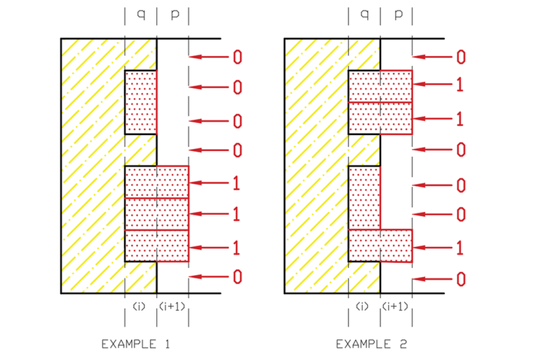
Here we can see two possible $$$p$$$ profiles for a fixed $$$q$$$ profile. From this, we can observe the following:
- If $$$q$$$'s $$$i^{th}$$$ bit value is $$$1$$$, then we can't place any tiles there, so $$$p$$$'s $$$i^{th}$$$ bit is always $$$0$$$.
- If $$$q$$$'s $$$i^{th}$$$ bit value is $$$0$$$, then we can place a horizontal tile which is equivalent to setting $$$p$$$'s $$$i^{th}$$$ bit value to $$$1$$$
- If $$$q$$$'s $$$i^{th}$$$ and $$$(i+1)^{th}$$$ bits are both 0, then we can place a vertical tile there which corresponds to setting $$$p$$$'s $$$i^{th}$$$ and $$$(i+1)^{th}$$$ bit value to $$$0$$$.
That way, if we know $$$dp[i][q]$$$ for a given $$$q$$$, we can recursively generate all possible $$$p$$$ using those rules. In particular, if we are in row $$$j$$$ and reach cases $$$1$$$ or $$$2$$$, we can then call for $$$search(j+1)$$$; or call $$$search(j+2)$$$ when we can go for case $$$3$$$ (see pseudocode below). Our $$$p$$$ will be ready as we hit the the final row of the grid, and then we can do the transition $$$dp[i+1][p]+=dp[i][q]$$$ like in the previous solution.
Note that for every $$$q$$$ you call search on, you will do at least $$$n$$$ recursive calls to reach the end, and for every extra recursive call you do (that is, when we call both $$$search(j + 2, i, p, q)$$$ and $$$search(j, i + 1, p \wedge (1 \ll j), q)$$$) we will be generating an extra valid $$$p$$$ for that $$$q$$$, so the number of recursive calls we're doing in total is $$$n$$$ + $$$[number$$$ $$$of$$$ $$$different$$$ $$$p]-1$$$. That way, if we want to know the values of $$$dp[i][mask]$$$ for column $$$i$$$ when we already calculated $$$dp[i-1][mask]$$$, we call search on all possible $$$q$$$ and obtain those values in $$$O(\sum_{q}$$$ $$$n$$$ + $$$[number$$$ $$$of$$$ $$$different$$$ $$$p]) = O(2^n \cdot n+C(n))$$$, which gives us an $$$O(m \times (2^n \cdot n+C(n)))$$$ algorithm in total.
Using the fact that this algorithm for generating valid $$$p$$$'s exists, we can also find a more satisfying bound for $$$C(n)$$$.
Let's try to estimate how many $$$p$$$ a fixed $$$q$$$ generates. We only generate extra $$$p$$$ when we call both $$$search(j+1)$$$ and $$$search(j+2)$$$, which happens when we have 2 adjacent $$$0$$$ on $$$q$$$'s binary representation. Note that the most number of recursive calls (that is, the most amount of different $$$p$$$) happens when all $$$0$$$ in $$$q$$$'s mask are adjacent, so we will only care about this case when calculating the upper bound for $$$C(n)$$$.
Let $$$totalcalls(i)$$$ be the total number of times we will call the $$$i^{th}$$$ adjacent $$$0$$$ in a certain $$$q$$$'s profile. We have that $$$totalcalls(1) = 1$$$, $$$totalcalls(2) = 1$$$ and for $$$n>2$$$ we have $$$totalcalls(n) = totalcalls(n-1) + totalcalls(n-2) = f_{n}(n_{th}~fibonacci~no.)$$$! Now we know that if $$$q$$$ has $$$k$$$ $$$0$$$'s in it's profile, the number of valid $$$p$$$ in it is bounded by $$$O(f_{k}) = O(\phi^{k}) \approx O(1.62^k)$$$. Here $$$\phi$$$ represents the Golden ratio.
There are $$$\binom{n}{k}$$$ masks with $$$k$$$ zeroes, so $$$C(n) = O(\sum_{k} \binom{n}{k} \cdot \phi^k ) = O((1+\phi)^n) \approx O(2.62^n)$$$. Plugging $$$n = 10$$$ into that gives us that $$$C(10) \approx 2.62^{10} = 15240$$$ which is a lot closer to the 5741 we found earlier.
That way, we have a $$$O(m \cdot n \cdot 2^n + 2.62^n \cdot m)$$$ solution for the recursive approach and a $$$O(4^n + 2.62^n \cdot m)$$$ solution for the approach mentioned previously using precalculation, both easily passing the time limit.
Our solution using precalculation is already as good as it gets, but we can optimize the recursive solution further. An intuition for why it can be done is that we may reach the same "situation" multiple times when doing recursive calls, where up to a certain row everything ends up tiled the same way despite the initial $$$q$$$ we call the recursion on being different. We will optimize that solution to $$$O(m \cdot n \cdot 2^n)$$$ using aforementioned broken profile dp, which will be the last optimization we see for this problem.
Optimization using Broken Profile DP
When we hit the base case during transitions as above; $$$p$$$ is already completely formed, but we can generate the same $$$p$$$ multiple times. Now the question arises, how can we store information about a profile that is not completely formed yet to avoid this scenario? Note that if we are generating the $$$j_th$$$ row of $$$p$$$, the bits on positions $$$0$$$ to $$$j$$$ of $$$q$$$ are useless from now on, and what will matter is only what bits we already formed from $$$p$$$ and what bits are still remaining in $$$q$$$.
That way, we will break the profile into "formed" and "not-yet-formed" parts by adding another state $$$j$$$ in our dp to keep track of up to what cell in our profile is "formed". Hence we have the name DP on broken profiles. Let's think of how we will define our dp by looking at some illustrations.
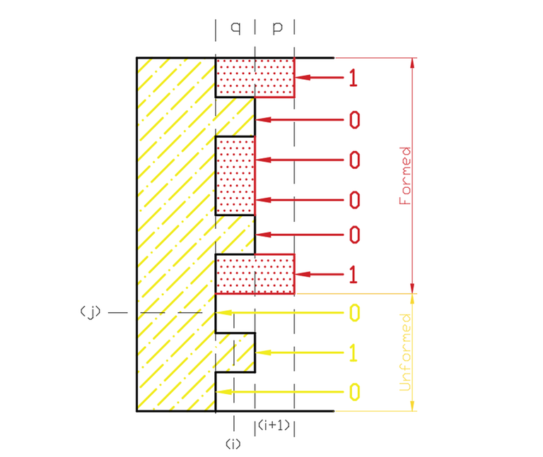
As mentioned earlier, we can see that in that the information we need to store are the bits we generated of $$$p$$$ that are in the formed part (in the above diagram the state of the formed part is $$$100001$$$) and that for the unformed part we need to store the bits remaining from $$$q$$$ (in the above diagram the state of it is $$$010$$$). That way, we define our dp state as $$$dp[i][j][x] = $$$ number of ways to fill grid's first $$$(i-1)$$$ columns and additionally fill the first $$$j$$$ rows of the $$$i^{th}$$$ column with profile $$$x$$$ sticking out into the next columns, $$$x$$$ being this junction of the unformed and formed parts of $$$p$$$.
This makes our transition from $$$j$$$ to $$$j+1$$$ and $$$q$$$ to $$$p$$$ way easier. Let's see how those transitions will take place, keeping in mind that we are filling $$$i^{th}$$$ column that peaks into the $$$(i+1)^{th}$$$ column.
Let's understand the cases of the recurrence:
- If the immediately next cell after formed part in the $$$i^{th}$$$ column is tiled (that is, $$$x~\And~2^{j+1}=1$$$), we can't put a horizontal tile there. That way, the transition will be $$$(i,j,x) \longrightarrow (i,j+1,x')$$$; where $$$x' = x - 2^{j+1}$$$ and $$$dp[i][j+1][x']+=dp[i][j][x]$$$
- If the immediately next cell after formed part in the $$$i^{th}$$$ column is not tiled (that is, $$$x~\And~2^{j+1}=0$$$), we can put a horizontal tile there. That way, we have the transition $$$(i,j,x) \longrightarrow (i,j+1,x')$$$ where $$$x' = x + 2^{j+1}$$$, and $$$dp[i][j+1][x']+=dp[i][j][x]$$$
- If we have two consecutive cells in the unformed part being $$$0$$$, we can put a vertical tile there too. In that scenario, both bits $$$(j+1)$$$ and $$$(j+2)$$$ of $$$x$$$ wouldn't change, since the profile on those rows would go from filling the $$$(i-1)^{th}$$$ column but not poking into the $$$i^{th}$$$ column to filling the $$$i^{th}$$$ column but not poking into the $$$(i+1)^{th}$$$ column. That way, the transition is $$$(i,j,x) \longrightarrow (i,j+2,x)$$$, and $$$dp[i][j+2][x]+=dp[i][j][x]$$$.
- The 3 transitions above are related to when $$$j < n$$$ and we're transitioning from $$$j$$$ to $$$(j+1)$$$ or $$$(j+2)$$$. For the transition from $$$i$$$ to $$$(i+1)$$$; if we look at the above diagram carefully; state $$$(i,n,x)$$$ for arbitrary $$$x$$$ is same as state $$$(i+1,0,x)$$$. A way to visualize it is thinking that the current column's red (formed) profile is next one's yellow (unformed) profile. That way, $$$dp[i+1][0][x] = dp[i][n][x]$$$.
Let us have a look at how to implement this approach.
Overall Time Complexity : $$$O(n \cdot m \cdot 2 ^ n)$$$
Link to CPP Code (iterative)
Link to CPP Code (recursive)
Link to Python Code (recursive)
Some external resources on DP on broken profiles that are worth visiting are USACO Guide Advanced Section, Broken Profile Dynamic Programming blog by evilbuggy and this video by Pavel Mavrin (pashka). I would also suggest reading the solution that has been taken up in the CSES Competitive Programmer's Handbook; which includes the formula that can be used to calculate the number of tilings in a more efficient manner. If some more curious reader is interested in reading the proof for the formula used, it can be found here.
Counting Numbers (2220)
This problem is a very standard application of Digit DP. Digit DP can be used to solve problems where we need to count the number of integers in a given range that follow a certain given condition. If you are new to this idea of digit dp, I would suggest reading the Digit DP section from this e-book to get a good introduction.
Our task in this problem is to count the number of integers between $$$a$$$ and $$$b$$$ where no two adjacent digits are the same. The naive approach will be to iterate through all the integers in the range $$$[a, b]$$$, but worst-case time complexity for that will be $$$O(1e18)$$$. The first observation that we need to make about this problem is that $$$ans[a, b] =$$$ $$$ans[0, b] -$$$ $$$ans[0, a - 1]$$$. Now, instead of solving for a range between two given integers, we have reduced the task to finding the answer for the range from $$$0$$$ to a given integer. But, instead of iterating over the numbers that satisfy our required condition, we can instead try to count in how many ways we generate such valid integers by building them from left to right. Let us try to find a proper dp state that we can use to count the number of ways of generating such numbers.
Let the task at hand be to find the number of valid integers in the range $$$[0, c]$$$ for some given integer $$$c$$$. Let the number of digits in $$$c$$$ be $$$n$$$. Let us define our dp state as $$$dp[n] =$$$ number of valid integers with $$$n$$$ digits.
Now, let us place a digit $$$d_{0}$$$ in the left most position of the number we are generating. Now our integer becomes $$$d_{0}[d_{1}d_{2}...d_{n}]$$$. Now we need to generate an integer of $$$(n - 1)$$$ digits, such the the left-most (leading digit) is $$$\neq$$$ $$$d_{0}$$$. In light of this, we can update our dp state to now be $$$dp[n][x] =$$$ number of valid integers with $$$n$$$ digits whose leading digit is $$$\neq$$$ x. Initially, any digit could have been the leading digit (for now, let us consider $$$0$$$ to be a valid leading digit); and hence our answer using this definition of our dp state will be $$$dp[n][-1]$$$.
Now we need to consider what happens when we have leading zeroes. Let the number we are generating be $$$d_{0}d_{1}d_{2}...d_{n}$$$. If we have $$$d_{0} = 0$$$ we can still put $$$d_{1} = 0$$$ because the integer has not yet started. For example, $$$000157 = 00157 = 157$$$. This essentially means that we can place as many consecutive leading zeroes as we want without making our integer invalid. Hence we will add a $$$3^{rd}$$$ parameter to our dp state, which will be a boolean, to check if we are still putting consecutive leading zeroes. By this new definition our dp state now becomes $$$dp[n][x][lz]$$$ where lz can be either $$$0$$$ or $$$1$$$. For the case of our answer, we have $$$dp[n][-1][1]$$$ since initially we can put leading zeroes.
Up until now, we are generating all valid integers that have $$$n$$$ digits; without the constraint of our integer being $$$\leq c$$$. For example, if we have $$$c = 157$$$, we are generating all valid integers upto $$$999$$$. If we have to keep our integer $$$\leq c$$$, we cannot place a digit in our generated integer that makes the resulting integer $$$> c$$$. For this purpose we introduce a $$$4^{th}$$$ parameter in our dp state: a flag called $$$tight$$$, which will be on if we didn't place a digit that makes the number $$$< c$$$ yet
Let us understand what this does with an example. Let us take $$$c = 4619$$$. Initially our tight constraint is $$$4$$$ since the leading digit in our integer cannot be $$$> 4$$$. If we place leading digit $$$d_{0} < 4$$$; then we are no more under a tight constraint since any number starting with $$$d_{0}$$$ will be less than $$$c$$$. But if we have $$$d_{0} = 4$$$, our tight constraint now changes to the second digit in $$$c$$$, which is $$$6$$$. Our new dp state now is $$$dp[n][x][lz][tight]$$$, where $$$tight$$$ is a boolean that tells us if we still have to follow the tight constraint of $$$c$$$. Our required answer now will be $$$dp[n][-1][1][1]$$$. We set $$$tight$$$ as $$$1$$$ as we need to think about the constraint that is the first digit of our input number.
We now take a look at how we transition between our dp states and obtain the answer.
- In the end, we have a dp with the following definition: $$$dp[n][x][lz][tight] =$$$ number of ways to generate a number of $$$n$$$ digits such that the leading digit is not $$$x$$$, can have multiple leading zeroes only if $$$lz = 1$$$ and must follow the constraints imposed by $$$c$$$ only if $$$tight = 1$$$
- When calculating a given $$$dp[n][x][lz][tight]$$$, test all possible first digits for that state: either from $$$0$$$ to $$$9$$$ if $$$tight = 0$$$ or from $$$0$$$ to the corresponding digit of $$$c$$$ if $$$tight = 1$$$. You need to check if that digit is either $$$\neq x$$$ or if that digit is $$$0$$$ and $$$lz = 1$$$.
- Let's say we are fixing that the current digit will be $$$d$$$. We will increase our dp by $$$dp[n-1][d][lz'][tight']$$$, where $$$lz'$$$ becomes $$$0$$$ if $$$d \neq 0$$$ and $$$tight$$$ becomes $$$0$$$ if $$$d < $$$ the corresponding digit on $$$c$$$.
- Finally we will use memoization to avoid recomputing the same states using our dp table. We have $$$O(10 \times 2^2 \times n) \approx O(10 \times n)$$$ states and for each state we test up to $$$10$$$ digits. The time complexity of this approach is $$$O(10^2 \times n)$$$ for each of the two calls for $$$a - 1$$$ and $$$b$$$, where $$$n$$$ is the number of digits of $$$a$$$ and $$$b$$$.
Link to $$$O(10^2\times n)$$$ Code
Bonus $$$O(n)$$$ solution: Let $$$c_i$$$ be the $$$i^{th}$$$ digit on $$$c$$$. Instead of calculating the dp, when we try figuring out how many numbers $$$< c$$$ follow the constraint, let's fix what is the first $$$i$$$ such that the $$$i^{th}$$$ digit of the generated number is $$$ < c_i$$$. If that is the case, we have either $$$c_i$$$ possibilities for its value (from $$$0$$$ to $$$c_i - 1$$$) if $$$c_{i-1} \geq c_i$$$ and $$$c_i-1$$$ otherwise (from $$$0$$$ to $$$c_i - 1$$$ except $$$c_{i-1}$$$), and for each of the following $$$n-i$$$ digits we have exactly $$$9$$$ choices (any of the $$$10$$$ possible digits except the one chosen on the previous one). That way, if we sum the corresponding answer for each valid $$$i$$$ (it could be that $$$c_j = c_{j+1}$$$, so choosing $$$i \geq j$$$ would lead to an invalid answer) and remember to take leading zeroes into account, we reach answer we wanted.
Please feel free to to share any suggestions, corrections or concerns.


Yay, it's out!
I spent a significant ammount of time trying to word things in a way that makes everything as clear as possible, so much time that i probably delayed the blog coming out XD.
I also recommend you take a look at Counting Tilings even if you are familiar with the problem, there are a lot of cool tricks there!
Hope you guys like it!
I upvoted. (Leo <3)
I upvoted too <3
Thank you boss. DP on profile was really great....
Thanks for the editorial.
The solutions(especially Counting Tilings) are really detailed! Definitely going to starred.
Amazing blog! Thank you for helping the community!
finally useful blog :D
after reading 648958435 blog about how be can pupil/specialist
In the problem "Elevator Rides", I used this approach.
"We start from weight = 0, and mask = 0 (meaning we haven't taken any person yet). Then in each recursion step, we iterate over all persons, check if the person has been already taken before or not, and move to
rec(weight + w[person], mask | (1 << person))if taking that person wouldn't exceed the weight by x otherwise move to1 + rec(w[person], mask | ( 1 << person))."Problem link: https://cses.fi/problemset/task/1653/
Submission link: https://cses.fi/paste/8f406e65ea0636015f4357/
Can Counting Numbers (2220) be solved in lesser dp states? (In first dp approach)
Nevermind. solved it with just 3 states:
link
Lmao I used Hadamard Transform the first time I solved Elevator Rides
for Elevator rides problem:
if (weight + peopleWeights[person] > x) {
                rides++;
                weight = min (peopleWeights[person], weight);
            }
Desicrption says "and the weight of the new last rides becomes the weight of the person being added:"
While the code is doing weight = min (peopleWeights[person], weight);?