


Hi Codeforces!
Today I want to tell you about a really cool and relatively unknown technique that is reminiscent of Centroid decomposition, but at the same time is also completely different.
The most common and well known decomposition tree algorithm out there is the centroid decomposition algorithm (running in $$$O(n \log n)$$$). It is a standard algorithm that is commonly used to solve tons of different kind of divide and conquer problems on trees. However, it turns out that there exists another closely related decomposition tree algorithm, that is in a sense optimal, and can be implemented to run in $$$O(n)$$$ time in around $$$30$$$ lines of code. I have chosen to call it the Shallowest Decomposition Tree. This blog will be all about the shallowest decomposition tree. Something I want to remark on before we start is that I did not invent this. However, very few people know about it. So I decided to make this blog in order to teach people about this super cool and relatively unknown technique!
I believe that part of the reason for why the shallowest decomposition tree is almost never used in practice is because no one has published a simple to use implementation of it. My contribution here is that I've come up with a slick and efficient implementation that constructs the decomposition in linear time. I've implemented it both in Python and C++.
Shallowest Decomposition Tree:
And for comparison, here are also a couple of centroid decomposition tree implementations using the same interface.
Centroid Decomposition Tree:
1. Motivation / Background
Take a look at the following problem

1.1. What exactly is a "decomposition tree"?
Think about how one could visualize a deterministic strategy in the treasure hunt game. One natural way to do it is to create a new tree where the root of this new tree is the first node you guess. The children of this root are all the possible 2nd guesses (which depend on the result of the first guess). Then do the same for 3rd guesses, 4th guesses, etc. I am going to refer to this resulting tree as a decomposition tree of the original tree. Note that the goal of minimizing the number of guesses is equivalent to constructing the shallowest possible decomposition tree.
1.2. The centroid guessing strategy
A natural strategy for the treasure hunt game is to guess the centroid of the tree. The definition of a centroid is a node, such that if removed from the tree, would split the tree into subtrees such that all subtrees have a size $$$\leq n/2$$$. Note that trees always have at least one centroid, and can have up to a maximum of 2 centroids.
In practice, a common way to find a centroid is to start at some arbitrary node $$$u$$$, try splitting the tree at $$$u$$$, and find the largest subtree from the split. If the size of the largest subtree is $$$> n/2$$$, then you move $$$u$$$ in the direction of that subtree. If the size of the largest subtree $$$\leq n/2$$$, then $$$u$$$ is a centroid, and so you have found a centroid.
By repeatedly guessing centroids in the treasure hunt problem, the set of nodes the treasure could be hidden at is guaranteed to decrease by at least a factor of $$$2$$$ for each guess. This will lead to having to do at most $$$\log_2(n)$$$ guesses in worst case. However, it turns out there examples of trees where this centroid guessing strategy is sub-optimal.
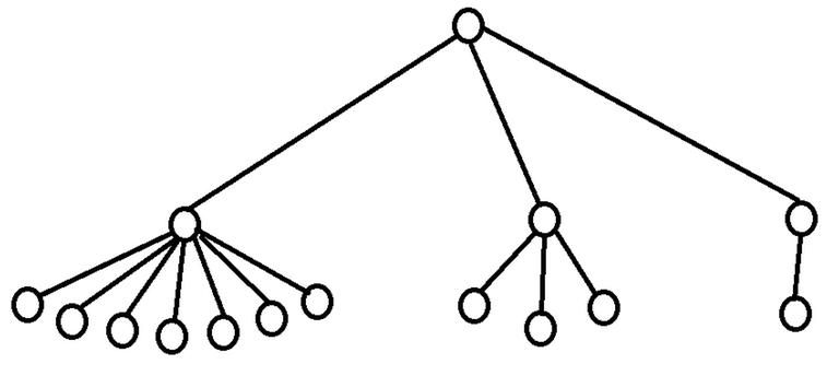
1.2.1. Examples of trees where the centroid guessing strategy is not optimal
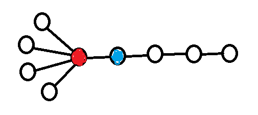
1.3. The center guessing strategy
Another natural strategy for the treasure hunt game is to guess the center of the tree, i.e. the least eccentric vertex (the "middle node" of the diameter). This turns out to be a fairly bad strategy, as can be seen in the following counter example (credit to dorijanlendvaj for this example).
2. Shallowest decomposition tree
Now we are finally at the point where we can talk about how to find the optimal (the shallowest) decomposition tree. The key to finding the shallowest decomposition tree turns out to be a greedy solution of a certain "Labeling Problem" 321C - Ciel the Commander.
It turns out that this labeling problem can be solved optimally by labeling greedily.
In the next section, we will prove that greedy labeling is in fact optimal, and we will also show how to construct it in linear time.
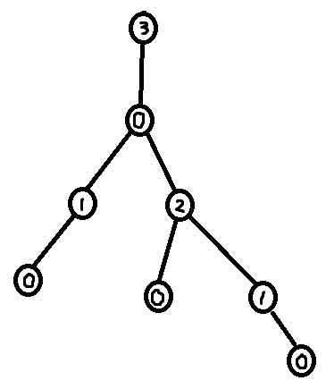
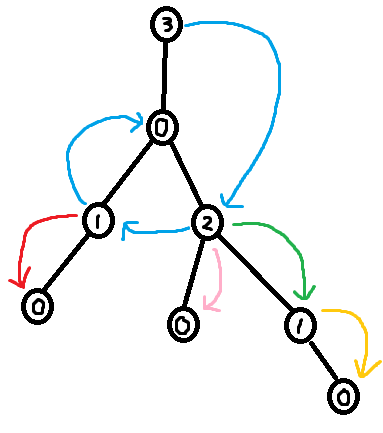
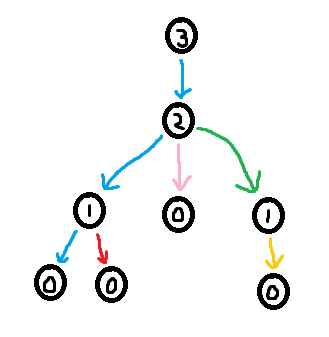
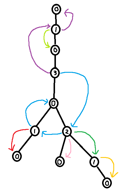
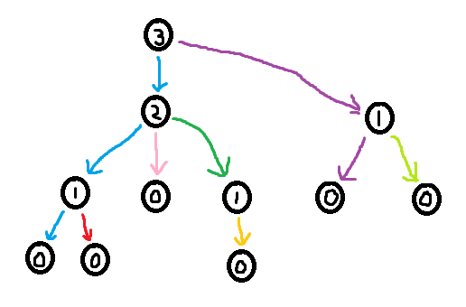
Something that is very important to note is that it is possible to extract a decomposition tree from a labeling. The highest labeled node must have a unique label (because of constraint 2). So start by picking the highest labeled node as the root for the decomposition. Then remove that node and recurse. This will lead to a decomposition tree of depth $$$\leq$$$ largest label.
Also note that given a decomposition tree it is possible to create a labeling. One way to do this is to label the nodes by their height in the decomposition tree. This will make it so the largest label used $$$=$$$ depth of the decomposition tree.
The take away from this discussion is that optimally solving the labeling problem is equivalent to finding an optimal deterministic strategy in the treasure hunt game, since a solution to the labeling problem can be made into a deterministic strategy for the treasure hunt game, and vice versa. So our (optimal) greedy labeling corresponds to an (optimal) deterministic guessing strategy in the treasure hunt game.
3. Analysis of greedy labeling
Let us first define the notion of forbidden labels. Given a rooted tree, a labeling of the tree, and a node $$$u$$$ in the tree, define forbidden(u) as the bitmask describing all labels that cannot be put on $$$u$$$ considering the descendants of $$$u$$$. I.e. bit $$$i$$$ of forbidden(u) is $$$1$$$ if and only if labeling node $$$u$$$ with label $$$i$$$ would cause a contradiction with the labels of the descendants of $$$u$$$.
Note that in the case of the greedy labeling, the label of $$$u$$$ corresponds to the least significant set bit of forbidden(u) + 1, or equivalently it is the number of trailing zeroes of forbidden(u) + 1.
3.1 A O(n) DP-algorithm for greedy labeling.
In the case of the greedy labeling, it is possible to make a DP-formula for forbidden(u). There are 3 cases:
Case 1. Node $$$u$$$ has no children. In this case forbidden(u) = 0.
Case 2. Node $$$u$$$ has exactly one child $$$v$$$. In this case forbidden(u) = forbidden(v) + 1.
Case 3. Node $$$u$$$ has multiple children, $$$v_1$$$, ..., $$$v_m$$$. In this case bit $$$i$$$ is set in forbidden(u) if either
bit $$$i$$$ is set in at least one of
forbidden(v_1) + 1, ...,forbidden(v_m) + 1.or there exists $$$j > i$$$ such that bit $$$j$$$ is set in at least two of
forbidden(v_1) + 1, ...,forbidden(v_m) + 1.
This gives us a simple O(n) implementation of the greedy labeling algorithm.
# Count trailing zeros
# Or equivalently, index of lowest set bit
def ctz(x):
    return (x & -x).bit_length() - 1

forbidden = [0] * n
def dfs(u, p):
    forbidden_once = forbidden_twice = 0
    for v in graph[u]:
        if v != p:
            dfs(v, u)
            forbidden_by_v = forbidden[v] + 1
            forbidden_twice |= forbidden_once & forbidden_by_v
            forbidden_once |= forbidden_by_v
    forbidden[u] = forbidden_once | (2**forbidden_twice.bit_length() - 1)
dfs(root, -1)
labels = [ctz(forbidden[u] + 1) for u in range(n)]
Remark: It is not actually obvious why this algorithm runs in linear time since this algorithm could in theory be using big integers. But as we will see in the next section, Section 3.2, greedy labeling is optimal. So by comparing the greedy labeling to centroid labeling, we know that the largest forbidden label for the greedy labeling is upper bounded by $$$\log_2(n)$$$. So this DP-algorithm does not use any big integers, and is therefore just a standard dfs algorithm which runs in linear time.
3.2 Greedy labeling is optimal
Lemma: Given a rooted tree (rooted at some node $$$r$$$). Out of all possibly labelings of this rooted tree, the greedy labeling (with root $$$r$$$) minimizes forbidden(r).
Note that minimizing forbidden(r) is effectively the same thing as minimizing the largest label used in the labeling. So it follows from this claim that the greedy algorithm uses the fewest number of distinct labels out of any valid labeling.
3.3. Adv. Constructing the shallowest decomposition tree in linear time
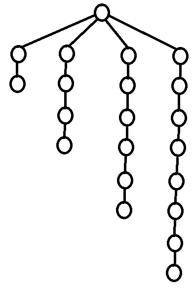
As seen in section 3.2, it is easy to construct the greedy labeling in linear time. However, it is far more tricky to construct the shallowest decomposition tree in $$$O(n)$$$ time. The way we will do it is by making use of chains. Before we formally define what a chain is, take a look at the following examples.
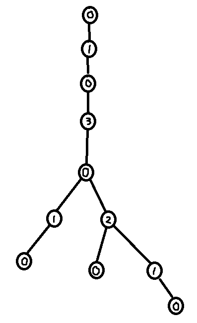
So formally,
Using the forbidden variable, it is possible to identify these chains. If $$$v$$$ is a child of $$$u$$$, then set of labels in forbidden(v) + 1 which are smaller than $$$u$$$'s label corresponds to a (Case 1) chain. Furthermore, the set of labels in forbidden(root) + 1 corresponds to the (Case 2) chain. So we can easily identify the sets of labels making up the chains. However, what we need in order to build the decomposition tree is to find the set of nodes that make up the chains.
The last trick we need is to use $$$O(\log n)$$$ stacks (one stack for each label). To extract the shallowest decomposition tree. Do a DFS over the greedily labeled tree. When we first visit a node, append that node into its corresponding stack. Furthermore, during the dfs, whenever we identify the labels of a chain, we can pop the corresponding stacks in order to find the nodes making up that chain. Then add the chain edges to the decomposition tree. I've called this popping procedure extract_chain in the code below.
With this, the linear time algorithm for the shallowest decomposition tree is finally complete! However, it is still possible to make some slight improvements. The main improvement would be to greedy label and build the decomposition tree at the same time in a single dfs, instead of using two dfs's. This is what I've chosen to do in my Python and C++ implementations found at the top of this blog. Another possible improvement is to have a variable for forbidden[u] + 1 instead of forbidden[u] itself. Because of comprehensibility, I've chosen not to do this. But it would definitely help if you'd want to codegolf it. The final possible improvement is to switch from using a recursive dfs to manually doing the dfs using a stack. This improvement is important for languages that don't handle recursion well, like Python.
4. Benchmarks
To my knowledge, every problem that can be solved with centroid decomposition can be solved with shallowest decomposition tree too, and you can freely switch between them. So here are a couple of comparisons between the two decompositions.
- 321C - Ciel the Commander
- Centroid (Python) TLE 1.34 s / 1 s | Shallowest (Python) 0.72 s | Centroid (C++) 0.28 s | Shallowest (C++) 0.16 s
- 914E - Palindromes in a Tree
- Centroid (Python) TLE 4.2 s / 4 s | Shallowest (Python) 3.75 s | Centroid (C++) 1.67 s | Shallowest (C++) 1.53 s
321C - Ciel the Commander is a good example of a problem where most of the time is spent building the decomposition tree. Here we can see a fairly significant boost from using the Shallowest Decomposition Tree compared to using Centroid Decomposition, especially if we take away the time spent on IO. 914E - Palindromes in a Tree is a good example of a problem where building the decomposition tree only takes up a small portion of the total time. For this reason, we only see a small performance gain from using the Shallowest Decomposition Tree.
Remark: There are definitely faster solutions to 321C - Ciel the Commander out there. For example, you could solve the problem just by outputting a greedy labeling without ever constructing any kind of decomposition tree. But the reason I'm using this problem as a benchmark is to compare the time used to construct the shallowest decomposition tree vs the centroid decomposition tree.
5. Mentions and final remarks
A big thanks Devil for introducing the shallowest decomposition tree to me. Also a big thanks to everyone that has discussed the shallowest decomposition tree with me over at the AC server. qmk magnus.hegdahl nor gamegame Savior-of-Cross meooow brunovsky PurpleCrayon.
One final thing I want to mention is that I know of two competitive programming problems that are intended to be solved specifically using the shallowest decomposition tree. Chronologically, the first problem is Cavern from POI. From what I understand, they were the first to come up with the idea. Many years later, atcoder independently came up with Uninity.
There has also been a much more recent problem 1444E - Finding the Vertex, which is a treasure hunt game on a tree, where you are allowed to guess edges instead of nodes. The solution isn't exactly the shallowest decomposition tree, but the method used to solve it is closely related to the shallowest decomposition tree. I challenge anyone that think they've mastered shallowest decomposition tree to solve it. If you need help on it, then take a look at my submission 242905032.


