


Part 1: [Tutorial] My way of understanding Dinitz's ("Dinic's") algorithm
Part 2: [Tutorial] Minimum cost (maximum) flow
Part 3: [Tutorial] More about minimum cost flows: potentials and Dinitz
Introduction
My philosophy on writing blogs is that I only write blogs when I feel that I have something new and interesting to contribute. This is usually not the algorithm itself, of course, but it can be that I recently found or heard of a new perspective or I figured out a way to explain something in a new way. This is in contrast to my dear colleagues at GeeksForGeeks who write the most low-effort (and often wrong) tutorial on everything and then sit at the top of Google results using their somehow world-class SEO.
This is one such case. I have an idea how to explain Dinitz's algorithm in a way I haven't heard of before (but it is not very hard to come up with, so this is not a claim to originality). In addition, this blog is a multi-parter, and in my next blog it is very convenient to start from the notions I establish here today.
The approach I am going to take is explaining the idea from a perspective of "the space of all possible changes". At any given step of the algorithm, we have a flow. We can choose a way to change the flow from this "space" and apply the change. If we detect there is no possible increasing change to the flow, the algorithm is terminated. The space of changes is such that any valid flow can be reached from any valid flow by applying just one change. This idea is almost geometrical and can in fact be thought of as wandering around within a convex shape in high-dimensional space.
I believe that this viewpoint gives a broader and more natural understanding of the algorithm and the "big picture" compared to more narrow explanations that look like "well we have flow and sometimes we add reverse edges and mumble mumble blocking flow". In addition this grounding allows us to see Dinitz as a direct improvement on Edmonds-Karp instead of them being merely vaguely reminiscent of one another. $$$~$$$
A note on names and spelling. The author writes his name as Dinitz (not Dinic) and it is pronounced /'dɪnɪts/, DIN-its (not /'dɑɪnɪk/ DYE-nick). The algorithm was originally published in a Soviet journal under the name Диниц. When the paper was translated to English, the author's name was transliterated as Dinic. The issue is that "Dinic" gives a wrong impression on how the name is supposed to be pronounced.
This problem is pretty common among ex-Soviet people and places whose names are now written in the Latin alphabet ("Iye", not "Jõe" was still on Google Maps well into the 2010s), so I felt like this should be clarified.
Basic definitions
I kind of expect you to know this already, but just so we are on the same page I will reiterate this part. However, I do believe that it is possible to learn maximum flow for the first time from this blog.
Please pay close attention to these instructions even if you are a frequent flow-er, as they may differ from any tutorial you've read before.
We work on a directed graph. Multiple edges are allowed and in fact it is kind of important, especially in the minimum cost case. For a vertex $$$v$$$, by $$$\delta^+ (v)$$$ and $$$\delta^- (v)$$$ I denote the set of outgoing and incoming edges of the vertex $$$v$$$.
Definition 1. A flow network is a directed graph $$$G = (V, E)$$$, where each edge has a nonnegative capacity. We formalize this by saying there is a map $$$c \colon\, E \to \mathbb{R}_{\ge 0}$$$.
Definition 2. Let two different vertices $$$s, t \in V$$$ be given; call them the source and sink, respectively. A flow is a map $$$f \colon\, E \to \mathbb{R}$$$, satisfying:
- Edge rule: For every edge $$$e$$$, $$$0 \le f(e) \le c(e)$$$: the flow on every edge is nonnegative, and no larger than the capacity of the edge.
- Vertex rule: For every vertex $$$v$$$ except $$$s$$$ and $$$t$$$, $$$\displaystyle \sum_{e \in \delta^+ (v)} f(e) = \displaystyle \sum_{e \in \delta^- (v)} f(e)$$$: the sum of the flows on incoming edges is equal to the sum of the flows on outgoing edges.
Some people like the metaphor of water in pipes. We model the network as a network of water pipes: each edge $$$e$$$ is a (one-directional, somehow) pipe that can take a flow of up to $$$c(e)$$$ liters per second, each vertex is a junction. Water is pumped into the junction $$$s$$$ and out of the junction $$$t$$$. The flow $$$f(e)$$$ represents the literal flow of water: $$$f(e)$$$ is the amount of water, in liters per second, running through the pipe $$$e$$$. We can check that this, intuitively, follows the definition of a flow given above:
- No pipe can have a negative amount of water going through it, and the amount of water flowing through a pipe can not exceed its capacity.
- Other than the source and the sink, what goes into a junction must go out of a junction, and no more can come out of a junction than what came in.
The figure below shows some examples of flows. In all figures of this blog, "$$$x/y$$$" written onto an edge means that the edge has flow $$$x$$$ and capacity $$$y$$$.
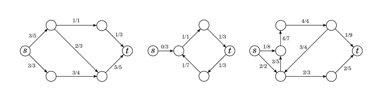
Perhaps particularly instructive is the second graph on the picture. It is a completely valid flow as the edge and vertex rules are satisfied. There is nothing wrong with the fact that there is some flow running around in a circle, not "coming" from $$$s$$$. Likewise, there is no rule that flow can't exit $$$t$$$ or enter $$$s$$$ from an edge.
The figure below shows some examples of invalid flows.
The first flow satisfies the edge rule, but the vertex rule is broken: in the top-left vertex, there is only 1 flow coming in, but $$$2 + 1 = 3$$$ flow coming out. The second flow satisfies the vertex rule, but the edge rule is broken: there is an edge with negative flow and an edge where the flow exceeds the capacity.
Definition 3. Given a flow network $$$(G, c, s, t)$$$ and a flow $$$f$$$, the value of the flow is
in other words, it is the amount of flow entering $$$s$$$ from an "outside source". It is possible to show that
Using the analogy of water pipes, it is the amount of water, in liters per second, pumped through the system.
Note that there is nothing in the definition that says the value of the flow must be nonnegative. In other words, this is also a valid flow:
It has negative value, -1 to be exact; it can be thought of as a positive flow from $$$t$$$ to $$$s$$$.
Definition 4. Given a flow network $$$(G, c, s, t)$$$, the maximum flow problem is to find a flow $$$f$$$ such that $$$\mathrm{val}(f)$$$ is maximized. Once again using the analogy of water pipes, it is the maximum amount of water, in liters per second, that we can pump from $$$s$$$ to $$$t$$$.
The residual network
Ford-Fulkerson, Edmonds-Karp and Dinitz are all greedy algorithms at heart. However, a naive greedy algorithm is wrong.
If your idea is simply to repeatedly find a path from $$$s$$$ to $$$t$$$ in the network and push as much flow through it as you can, then you will fail to the classical problem of greedy algorithms: early choices, even ones that seem good, will ruin important choices later. Consider this example:
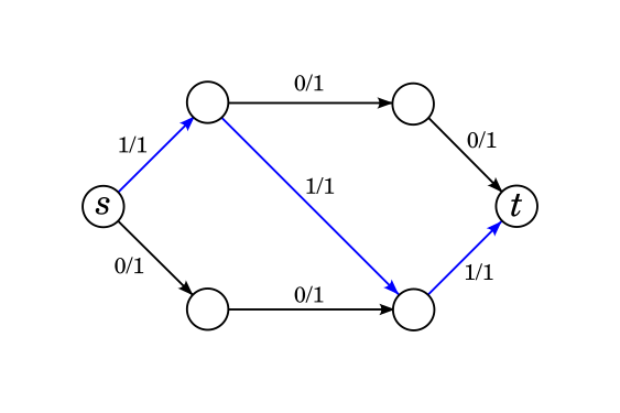
Suppose we tried this idea and sent flow through the blue path. It is impossible to find a new path to send flow through but it is easy to see that the actual maximum flow of this network is 2, not 1. We need to design the algorithm in such a way that if we do make this choice, there is a way for us to "unchoose" that diagonal edge later.
More generally, we need to formulate our greedy algorithms in a way that does not allow us to block good choices later. In fact, it would be awesome if we could design our algorithms in a way that earlier steps don't block any choices later.
Let $$$(G, c, s, t)$$$ be a flow network and $$$f, f'$$$ be flows. What do we know about the function $$$f' - f \colon\, E \to \mathbb{R}$$$, defined as $$$(f' - f)(e) = f'(e) - f(e)$$$?
- $$$-f(e) \le (f' - f)(e) \le c(e) - f(e)$$$, obtained by taking the vertex rule for $$$f'$$$ and subtracting $$$f(e)$$$ from both sides.
- For any vertex $$$v$$$ other than $$$s$$$ or $$$t$$$, $$$\displaystyle \sum_{e \in \delta^+(v)} (f' - f)(e) = \displaystyle \sum_{e \in \delta^- (v)} (f' - f)(e)$$$.
- If we define $$$\mathrm{val}(f' - f)$$$ the same way as we did for flows, $$$\mathrm{val}(f' - f) = \mathrm{val}(f') - \mathrm{val}(f)$$$.
The function $$$f' - f$$$ is almost like a flow: the vertex rule still holds perfectly. The edge rule also kind of holds except for the fact that instead capacities, we have an interval of possible valid values the flow on $$$e$$$ can take.
Definition 5. Given a flow network $$$(G, c, s, t)$$$ and a flow $$$f$$$, any function $$$g \colon\, E \to \mathbb{R}$$$ satisfying the following condition is called a flow difference w.r.t $$$f$$$:
- Edge rule: $$$-f(e) \le g(e) \le c(e) - f(e)$$$.
- Vertex rule: $$$\displaystyle \sum_{e \in \delta^+(v)} g(e) = \displaystyle \sum_{e \in \delta^-(v)} g(e)$$$.
We have already proven that given two different flows $$$f$$$ and $$$f'$$$, their difference $$$f' - f$$$ is a flow difference. The converse also holds:
Exercise 6. Prove that given a flow network $$$(G, c, s, t)$$$, a flow $$$f$$$ and a flow difference $$$g$$$ w.r.t. $$$f$$$, the function $$$f + g \colon\, E \to \mathbb{R}$$$ is again a flow on $$$(G, c, s, t)$$$.
The set of flow differences w.r.t. $$$f$$$ represents the set of possible changes we can make to $$$f$$$. Given any other flow, we can find a flow difference that takes us to that other flow, and any flow difference takes us to a valid flow. If we choose the things we do in the greedy algorithm from the set of flow differences, we never have to worry about blocking good choices later.
The concept of a flow difference has one downside: some edges have negative flow. In principle there is nothing wrong with that, but in what follows it is more convenient if flow is always nonnegative. We want to model negative flow as a flow in the other direction.
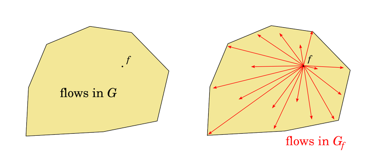
Definition 7. Given a flow network $$$(G, c, s, t)$$$ and a flow $$$f$$$, the residual flow network $$$G_f$$$ is a flow network defined as follows:
- The vertex set, source and sink vertices remain as they are.
- The edge set and its capacities are defined like this. For each edge $$$e$$$ from $$$u$$$ to $$$v$$$:
-
- If $$$f(e) < c(e)$$$, $$$G_f$$$ has an edge $$$e$$$ from $$$u$$$ to $$$v$$$ with capacity $$$c_f(e) = c(e) - f(e)$$$.
-
- If $$$0 < f(e)$$$, $$$G_f$$$ has an edge $$$\overleftarrow{e}$$$ from $$$v$$$ to $$$u$$$ with capacity $$$c_f(\overleftarrow{e}) = f(e)$$$.
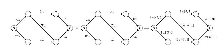
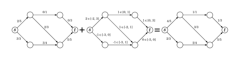
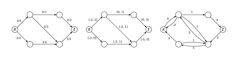
Below is a flow $$$f$$$, the range of allowed flows in a flow difference, and the residual network $$$G_f$$$.
Flow differences w.r.t. $$$f$$$ and flows in $$$G_f$$$ are virtually the same thing. Any flow $$$g$$$ in $$$G_f$$$ can be transformed into a flow difference $$$g'$$$ w.r.t $$$f$$$ by setting $$$g'(e) = g(e) - g(\overleftarrow{e})$$$ (if $$$e$$$ or $$$\overleftarrow{e}$$$ doesn't exist, then we count $$$g$$$ of that as zero).
Similarly, any flow difference $$$g'$$$ w.r.t. $$$f$$$ can be transformed into a flow $$$g$$$ in $$$G_f$$$ by
- $$$g(e) = \max(0, g'(e))$$$ if $$$e$$$ exists in $$$G_f$$$;
- $$$g(\overleftarrow{e}) = \max(0, -g'(e))$$$ if $$$\overleftarrow{e}$$$ exists in $$$G_f$$$.
For a flow $$$f$$$ in $$$G$$$ and a flow $$$g$$$ in $$$G_f$$$, $$$f + g$$$ can be defined through flow differences and it will be a valid flow in $$$G$$$. For flows $$$f'$$$ and $$$f$$$ in $$$G$$$, $$$f' - f$$$ can be defined through flow differences and it will be a valid flow in $$$G_f$$$.
So all that stuff we said about flow differences still holds for the residual network. The residual network $$$G_f$$$ also represents the set of possible changes we can make to $$$f$$$ while still letting it remain a valid flow.
One way to look at flows is to imagine flows as points in a massive, $$$|E|$$$-dimensional space. The $$$i$$$-th coordinate is the amount of flow on the $$$i$$$-th edge. The equalities and inequalities of the vertex and edge rules define the set of valid flows as a subset of this space, which is in fact a polyhedron. Flows in $$$G_f$$$ are exactly the vectors such that $$$f$$$ translated by the vector is still in the polyhedron.
Alternatively, replacing $$$G$$$ with $$$G_f$$$ is like changing the point of origin in this space. The polyhedron stays the same, but the point we have designated as $$$0$$$ changes.
By the way, this is not some kind of metaphor or intuitive picture. Flows really are points in $$$|E|$$$-dimensional space and the set of valid flows really is a convex polyhedron (in fact a polytope). To learn more about this kind of viewpoint, read about linear programming.
The Universal Max-Flow Algorithm template
What we now know can be assembled into an algorithm... almost. There is one step that is not described explicitly.
Algorithm 8. Given a flow network $$$(G, c, s, t)$$$.
- Initialize $$$f$$$ by setting $$$f(e) \gets 0$$$ for all edges. This is a valid flow.
- While $$$t$$$ is reachable from $$$s$$$ in $$$G_f$$$:
-
- Find some flow $$$\Delta f$$$ in $$$G_f$$$.
-
- Let $$$f \gets f + \Delta f$$$.
- Return $$$f$$$.
We have already pretty much proven that this algorithm solves the maximum flow problem. We have shown that throughout this process, $$$f$$$ is a valid flow. If $$$t$$$ is not reachable from $$$s$$$ in $$$G_f$$$, then there is no flow in $$$G_f$$$ with positive value, so we must be at a maximum.
All that is left to do is to specify how to find a flow $$$\Delta f$$$ in $$$G_f$$$. If we specify that, all that is left is to prove that the algorithm terminates and we have a valid max-flow algorithm.
Ford-Fulkerson algorithm. To find a flow $$$\Delta f$$$ in $$$G_f$$$, find a path from $$$s$$$ to $$$t$$$ in $$$G_f$$$. This is guaranteed to exist by the while-condition. Take the minimum capacity in $$$G_f$$$ along this path. Capacities in $$$G_f$$$ are positive, so this minimum capacity is also positive. Send this much flow through each edge on this path. If capacities are integer or rational, this definitely terminates.
Edmonds-Karp algorithm. Do literally the exact same thing as Ford-Fulkerson except that you take the shortest path from $$$s$$$ to $$$t$$$. How did it take two people to come up with that?
Dinitz's algorithm
Let $$$(G, c, s, t)$$$ be a flow network and $$$f$$$ a flow. We will describe Dinitz's way to find a flow in $$$G_f$$$.
Throw out some edges in $$$G_f$$$ so that we are left with a DAG $$$D$$$ where $$$s$$$ is a source and $$$t$$$ is a sink. There is definitely a way to do this: a path from $$$s$$$ to $$$t$$$ is suitable.
Finding a flow in $$$D$$$. This algorithm is best described in pseudocode.
We start with a slow algorithm and then work our way towards a better one.
 1 # a call to this function tries to push F flow from u
 2 # the return value is how much flow could actually be pushed
 3 function dinitz_dfs (u, F):
 4   if u == t:
 5     return F
 6   flow_pushed = 0
 7   for each edge e from u in the current DAG:
 8     dF = dinitz_dfs(e.v, min(F, e.capacity - e.flow))
 9     # turns out dF flow can be pushed from this vertex to the next
10     # push that much
11     flow_pushed += dF
12     F -= dF
13     e.flow += dF
14   return flow_pushed
15
16 dinitz_dfs(s, INF)
Essentially, this algorithm is a simple greedy idea. It does have a major shortcoming though. A lot of the time, the dinitz_dfs(u, F) is just going to return 0, doing no useful work whatsoever because no flow gets actually pushed. The next time we are in the same vertex, we are going to go through all of that again; since we only add flow and never remove it, we still can't push any flow from that vertex. This quickly becomes exponential much the same way as a naive DP without memoization does.
And the solution is much the same as well. We say an edge is blocked if it has reached its capacity. And we say a vertex is blocked if no flow can be pushed from it anymore: each edge going out from it is either blocked itself or the vertex at the other end is blocked. We can set these flags on the fly when we detect them. This leads to a much faster algorithm:
 1 # a call to this function tries to push F flow from u
 2 # the return value is how much flow could actually be pushed
 3 function dinitz_dfs (u, F):
 4   if u == t:
 5     return F
 6   flow_pushed = 0
 7   all_blocked = true
 8   for each edge e from u in the current DAG:
 9     if e.capacity != e.flow and !e.v.blocked:
10       dF = dinitz_dfs(e.v, min(F, e.capacity - e.flow))
11       # turns out dF flow can be pushed from this vertex to the next
12       # push that much
13       flow_pushed += dF
14       F -= dF
15       e.flow += dF
16
17     # separate if because the edge or the vertex might become
18     # blocked as a result of our actions above
19     if e.capacity != e.flow and !e.v.blocked:
20       all_blocked = false
21
22   if all_blocked:
23     u.blocked = true
24   return flow_pushed
25
26 dinitz_dfs(s, INF)
Update 19.07.2022: There are two more quick optimizations we can do here. Notice that on line 10, either we run out of $$$F$$$ or we block the edge (either by filling the edge to its capacity or by blocking the other endpoint). In the first case, we can break early. In the second, there is no need to consider that edge anymore during the current run of dinitz_dfs (we can somehow implement removing the edge, for example by storing the index of the first unblocked edge for every vertex). This has some interesting implications for complexity analysis. Every edge is blocked at most once and never reconsidered again. Every call to dinitz_dfs(u, F) results in blocking some edges and pushing flow through at most one edge without blocking it. Thanks to dacin21 for pointing this out.
This algorithm is often called the blocking flow algorithm or called "finding the blocking flow".
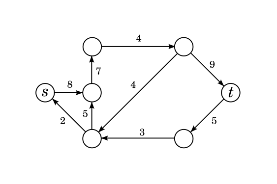
Choosing the DAG $$$D$$$. The DAG used in Dinitz's algorithm is what has been called the BFS subgraph or layered network. First, we consider only the vertices that are reachable from $$$s$$$ and from which $$$t$$$ is reachable. Then, we run a breadth-first search from $$$s$$$; this will calculate the distance (in number of edges) from $$$s$$$ to any given vertex. We add to the DAG all edges that go from one distance to the next. Something like this:
 1 function dinitz_bfs ():
 2   Q = {s} # a queue
 3   dist[s] = 0
 4   while Q is not empty:
 5     u = front of the queue
 6     pop the queue
 7   for each edge e from u:
 8     if dist[e.v] = undefined:
 9      dist[e.v] = dist[u] + 1
10      push v to the queue
11    if dist[e.v] = dist[u] + 1:
12      add e to the DAG
This is sometimes called a layered network because the graph is organized into layers, with $$$s$$$ in the first, $$$t$$$ in the last, and all edges go from one layer to the next.
Below is a possible example of a result. The black, solid edges are part of the DAG. The lighter, dashed edges were part of the graph, but aren't part of the DAG. The "layers" of the graph are also visually distinguished in the figure. All edges in the DAG go from one layer to the next; edges not in the DAG stay in the same layer or go back. Notice that there are no edges that go forward multiple layers, part of the DAG or not.
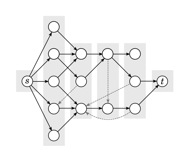
From the point of view of the correctness of the algorithm, this "layered" structure is not important: it's not even very important that the graph is a DAG, although it does make it easier to not worry about infinite loops in the DFS portion of the algorithm. The structure becomes important when analyzing the complexity, very similarly how replacing Ford-Fulkerson with Edmonds-Karp makes the algorithm run in polynomial time.
And with these two steps specified, that completes the description of the algorithm. If you want to see it in a "packaged" form, it looks like this:
Algorithm 9. Given a flow network $$$(G, c, s, t)$$$.
- Initialize $$$f$$$ by setting $$$f(e) \gets 0$$$ for all edges. This is a valid flow.
- While $$$t$$$ is reachable from $$$s$$$ in $$$G_f$$$:
-
- Construct the graph $$$D$$$ by doing a BFS from $$$s$$$ (
dinitz_bfs).
- Construct the graph $$$D$$$ by doing a BFS from $$$s$$$ (
-
- Use the blocking-flow algorithm (
dinitz_dfs) to find a flow $$$\Delta f$$$ in $$$D \subseteq G_f$$$.
- Use the blocking-flow algorithm (
-
- Let $$$f \gets f + \Delta f$$$.
- Return $$$f$$$.
And there you have it.
Finally, I should say one or two words about complexity. Complexity analysis of maximum flow algorithms is often kind of bogus because it is hard to find hard cases, and even if you do, in actual problems you usually aren't given an arbitrary network. Instead, you get to design your own which in all likelihood won't be the really, really bad case.
However, complexity analysis of maximum flow algorithms is a deep subject and I hope to write more about it at some point. For now, I will say this much. Let $$$n$$$ be the number of vertices and $$$m$$$ the number of edges.
One intuitive way to understand why this algorithm should be faster than Ford-Fulkerson or Edmonds-Karp is to think about it like this. In Edmonds-Karp, we pick one shortest path from $$$s$$$ to $$$t$$$; the Edmonds-Karp algorithm is known to work in time $$$O(m^2 n)$$$. In Dinitz, we do the same thing, but work on many shortest paths at the same time. This should be better, as we can avoid duplicated work in many cases. Consider a simple example where the shortest-paths graph looks like this:
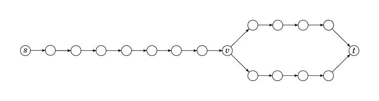
In the Edmonds-Karp case, we first traverse the path from $$$s$$$ to $$$t$$$ in the upper branch, then the path from $$$s$$$ to $$$t$$$ in the lower branch. All edges between $$$s$$$ and $$$v$$$ get traversed twice. By contrast, with Dinitz the edges between $$$s$$$ and $$$v$$$ get traversed only once, and the DFS splits the flow after that between the two branches.
Now imagine what happens if there are not two but a thousand branches that look like this.
Of course, this is just one example. In general though:
- The main loop is entered $$$O(n)$$$ times.
- The
dinitz_bfsruns in $$$O(m)$$$ time. - The
dinitz_dfsruns in $$$O(nm)$$$ time. - Calculating $$$f \gets f + \Delta f$$$ takes $$$O(m)$$$ time.
The first and third points are not trivial. They're not mega-hard either, but I wouldn't say that you can tell simply by looking at it. I won't be proving it right now. Within the loop, dinitz_dfs clearly dominates, so the time complexity is $$$O(n^2 m)$$$.
Finally, because there is a lot going on here, I have provided an implementation. Keep in mind that this implementation is mainly for educational purposes and is not necessarily optimized for constant factor. But in any case, you can refer to my code, I think you'll find there are ample comments. Code.


Thank you for writing this. I notice that I missreading it for a long time until see your blog.
One nice thing you could get from considering flow differences is when you subtract two flows of the same value from each other. It would be a flow of value $$$0$$$ in the residual network, which, in turn may be represented as a set of cycles (circulation).
It allows to e.g. classify all edges and vertices based on whether they can, can't or must be used in a flow of particular size (e.g. maximum flow) by looking on whether they lie on a cycle. One of possible problems that ask to do so, applied to perfect matching, is Timus 1676. Mortal Kombat.
What do you think is the faster flow algorithm? Push-relabel or dinitz with scaling?
Dude how insecure are you? Why do You have to insult Geeks for Geeks before your “amazing insights”?
Although I appreciate your blog on throwing new perspective/ideas on complex (atleast to me) algorithms such as the max flow algorithm you described in this blog (and these indeed takes lot of effort to organize and articulate to an extended community of developers), I have serious objection on the following statement:
"This is in contrast to my dear colleagues at GeeksForGeeks who write the most low-effort (and often wrong) tutorial on everything"
Well, that is a sweeping, broad brush generalization...
You read it wrong. He claims they write tutorials about everything.
Not often wrong on everything. Tutorial on everything.
I understand that I came off as rude but the reason I wrote that is that I'm frankly fed up with them. Because every time I Google something, they are up there, taking up space, overshadowing more deserving resources (note, I'm not saying my blog is necessarily one of them).
I have worked as a developer, and you're right, it's not just competitive programming. And it's also not just GeeksForGeeks. Often when I Google something, there are dozens of such sites that I have to sift through before I find anything useful. TutorialsPoint, C-Sharp Corner, you name it. If it were just one site, it might be easy to say that you can just ignore it, but there are so many of them that I can't even keep up with them. And it's not that I have some kind of specific question that not every site should answer. I have never gotten any help from these. Worst of the worst is JavaScript, literally impossible to Google about without appending "developers.mozilla" (and/or domain name of your favorite framework) to the search.
My resentment probably grew more during my work as a developer, because I had to Google more.
And please don't say, "well, but you're not a beginner...". I have been a beginner too, it was not that long ago. Even if not in CP, I have had to take up some new programming languages which effectively means that I will be looking up initialization of a vector too.
Now about "often wrong". Well, I'm not going to lie that I've conducted some sort of statistical survey of their accuracy. It's just that there are enough stories about them presenting $$$O(nm)$$$ solutions to TSP or mistakes in their sample implementations.
Yes, probably I should not have ranted about that in the introduction of an unrelated blog. I'm sorry. But it's hard to resist the temptation.
Thank you for your clarification and the detailed explanation.
I think your implementation has a worst-case running time of $$$\Omega(n\, m^2)$$$ as your
dinitz_dfsalways visits all the outgoing edges of the current vertex.The main idea is to take an anti-Edmonds-Karp case that produces $$$\Omega(V E)$$$ augmenting paths and attach an additional dense part with $$$O(E)$$$ edges near the sink.
The typical $$$O(n^2 m)$$$ implementation (a) maintains a current arc for every vertex (to avoid reconsidering already saturated edges) and (b) returns once a recursive call returned non-zero flow, i.e once $$$\mathrm{dF} > 0$$$ (and repeatedly calls
dinitz_dfs(s, INF)). (Side note: For (b) there's an optimization where we only return once $$$F$$$ hits zero, but I won't go into this. It basically helps if there is a long (dummy) path from the source, but not if there is a long (dummy) path to the sink.)For this "typical" implementation, I find the running-time analysis quite intuitive: Whenever we reach the sink, we return all the way to $$$s$$$ and in essence augment along the found path, so we basically find shortest augmenting paths in $$$O(n)$$$ time, compared to the $$$O(m)$$$ time (bfs) needed in Edmonds-Karp. This is why Dinitz runs in $$$O(n^2 m)$$$ while Edmonds-Karp runs in $$$O(n\, m^2)$$$. (The additional "bookkeeping" time spent advancing the current edges is $$$O(n\, m)$$$ as it's basically one DFS per phase. Similarly the dinitz_BFSs also takes $$$O(n\, m)$$$ time in total.) In fact, this shows that Dinitz finds augmenting paths of length $$$k$$$ in $$$O(k)$$$ time each, which gives some indication why the algorithm is often fast in practice. (Once again ignoring the $$$O(n\, m)$$$ bookkeeping time.)
Thanks. I was aware of this but I kind of forgot and kind of wanted to not overload the blog with too much information. But if it affects complexity then it deserves to be there.
Maybe add few words about capacity scaling at the end of the tutorial?
"Iterate $$$2^k{\downarrow}$$$, run the same dinitz which consider only edges with $$$c-f\ge2^k$$$, profit, $$$O(nm \log U)$$$"
bool exists (int u) { return capacity(u) >= (1 << k); }in your implementation.I thought that flow must come from s but in this article you said : "There is nothing wrong with the fact that there is some flow running around in a circle, not "coming" from s" which make me so confused @@ Did I misunderstand flow from the beginning?
You may be confused because the word “flow” can refer to slightly different things.
Generally, a network is a graph with capacities assigned to edges, and a flow in a network is a function that assigns a flow through each edge, subject to the edge condition (flow at each edge must be between 0 and the capacity of the edge) and the vertex condition (for each vertex apart from the source and sink, the flow into the vertex must equal the flow out of the vertex).
When talking about a maximum flow algorithm, the word flow refers not to a function, but to a scalar value: the net flow from the source vertex to the sink vertex.
So a flow in the first sense can have useless cycles that do not contribute to the flow in the second sense. It's technically true that if you have a maximum flow (in the second sense) you can add arbitrary useless cycles to it, subject to residual capacities, and it will still be a valid maximum flow in the first sense. However, most maximum flow algorithms, including Dinitz's algorithm which is explained here, do not generate useless flows like that.