


Introduction
There are a number of "small" algorithms and facts that come up again and again in problems. I feel like there I have had to explain them many times, partly because there are no blogs about them. On the other hand, writing a blog about them is also weird because there is not that much to be said. To settle these things "once and for all", I decided to write my own list about about common "small tricks" that don't really warrant a full tutorial because they can be adequately explained in a paragraph or two and there often isn't really anything to add except for padding.
This blog is partly inspired by adamant's blog from a few years ago. At first, I wanted to mimic adamant's blog structure exactly, but I found myself wanting to write longer paragraphs and using just bolded sentences as section headers got messy. Still, each section is short enough that it would not make much sense to write separate blogs about each of these things.
All of this is well-known to some people, I don't claim ownership or novelty of any idea here.
1. Memory optimization of bitset solutions
In particular, reachable nodes in a DAG. Consider the following problem. Given a DAG with $$$n$$$ vertices and $$$m$$$ edges, you are given $$$q$$$ queries of the form "is the vertex $$$v$$$ reachable from the vertex $$$u$$$". $$$n, m, q \le 10^5$$$. The memory limit does not allow $$$O(n^2)$$$ or similar space complexity. This includes making $$$n$$$ bitsets of length $$$n$$$.
A classical bitset solution is to let $$$\mathrm{dp}[v]$$$ be a bitset such that $$$\mathrm{dp}[v][u] = 1$$$ iff $$$v$$$ is reachable from $$$u$$$. Then $$$\mathrm{dp}[v]$$$ can be calculated simply by taking the bitwise or of all its immediate predecessors and then setting the $$$v$$$-th bit to 1. This solution almost works, but storing $$$10^5$$$ bitsets of size $$$10^5$$$ takes too much memory in most cases. To get around this, we use 64-bit integers instead of bitsets and repeat this procedure $$$\frac{n}{64}$$$ times. In the $$$k$$$-th phase of this algorithm, we let $$$\mathrm{dp}[v]$$$ be a 64-bit integer that stores whether $$$v$$$ is reachable from the vertices $$$64k, 64k + 1, \ldots, 64k + 63$$$.
In certain circles, this problem has achieved a strange meme status. Partly, I think it is due to how understanding of the problem develops. At first, you don't know how to solve the problem. Then, you solve it with bitsets. Then, you realize it doesn't work and finally you learn how to really solve it. Also, it is common to see someone asking how to solve this, then someone else will always reply something along the lines of "oh, you foolish person, don't you realize it is just bitsets?" and then you get to tell them that they're also wrong.
Besides the classical reachability problem, I also solved AGC 041 E this way.
2. Avoiding logs in Mo's algorithm
Consider the following problem. Given an array $$$A$$$ of length $$$n$$$ and $$$n$$$ queries of the form "given $$$l$$$ and $$$r$$$, find the MEX of $$$A[l], \ldots, A[r]$$$". Queries are offline, i.e. all queries are given in the input at the beginning, it is not necessary to answer a query before reading the next one. $$$n \le 10^5$$$.
The problem can also be solved with segment trees avoiding a square-root factor altogether. In this blog however, we consider Mo's algorithm. Don't worry, this idea can be applied in many situations and a segment tree solution might not always be possible.
A first attempt at solving might go like this. As always, we maintain an active segment. We keep a set<int> of all integers up to $$$n$$$ that are not represented in the active segment, and an auxiliary array to count how many times each number appears in the active segment. In $$$O(\log n)$$$ time we can move an endpoint of the active segment, and in $$$O(\log n)$$$ time we can find the MEX of the active segment. We move the endpoints one by one to go through all queries, and if the queries are sorted in a certain magical order, we get $$$O(n \sqrt n \log n)$$$ complexity. Unfortunately, this is too slow; also $$$O(n \sqrt n \log n)$$$ is an altogether evil complexity and should be avoided at all costs.
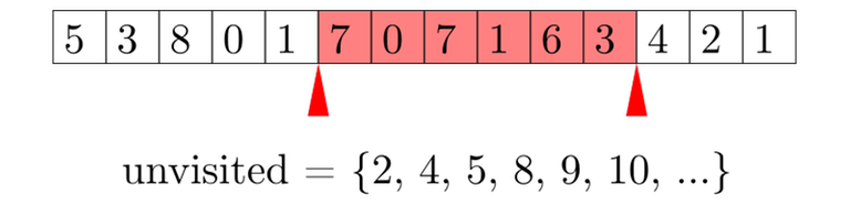
Clearly, set<int> is a bottleneck. Why do we use it? We need to support the following operations on a set:
- Insert an element. Currently $$$O(\log n)$$$. Called $$$O(n \sqrt n)$$$ times.
- Remove an element. Currently $$$O(\log n)$$$. Called $$$O(n \sqrt n)$$$ times.
- Find the minimum element. Currently $$$O(\log n)$$$. Called $$$O(n)$$$ times.
Note that operations 1 and 2 are more frequent than 3, but they take the same amount of time. To optimize, we should "balance" this: we need 1 and 2 to be faster, but it's fine if this comes at the expense of a slightly slower operation 3. What we need is a data structure that does the following:
- Insert an element in $$$O(1)$$$.
- Delete an element in $$$O(1)$$$.
- Find the minimum element in $$$O(\sqrt n)$$$.
This should be treated as the main part of the trick: to make sure endpoints can be moved in $$$O(1)$$$ time, potentially at the expense of query time. How the data structure actually works is actually even not that important; in a different problem, this data structure might be something different.
3. Square root optimization of knapsack/"$$$3k$$$ trick"
Assume you have $$$n$$$ rocks with nonnegative integer weights $$$a_1, a_2, \ldots, a_n$$$ such that $$$a_1+a_2+\cdots+a_n = m$$$. You want to find out if there is a way to choose some rocks such that their total weight is $$$w$$$.
Suppose there are three rocks with equal weights $$$a, a, a$$$. Notice that it doesn't make any difference if we replace these three rocks with two rocks with weights $$$a, 2a$$$. We can repeat this process of replacing until there are at most two rocks of each weight. The sum of weights is still $$$m$$$, so there can be only $$$O(\sqrt m)$$$ rocks (see next point). Now you can use a classical DP algorithm but with only $$$O(\sqrt m)$$$ elements, which can be lead to a better complexity in many cases.
This trick mostly comes up when the $$$a_1, a_2, \ldots, a_n$$$ form a partition of some kind. For example, maybe they represent connected components of a graph. See the example.
4. Number of unique elements in a partition
This is also adamant's number 13, but I decided to repeat it because it ties into the previous point. Assume there are $$$n$$$ nonnegative integers $$$a_1, a_2, \ldots, a_n$$$ such that $$$a_1 + a_2 + \cdots + a_n = m$$$. Then there are only $$$O(\sqrt m)$$$ distinct values among $$$a_1, a_2, \ldots, a_n$$$.
5. Removing elements from a knapsack
Suppose there are $$$n$$$ rocks, each with a weight $$$w_i$$$. You are maintaining an array $$$\mathrm{dp}[i]$$$, where $$$\mathrm{dp}[i]$$$ is the number of ways to pick a subset of rocks with total weight exactly $$$i$$$.
Adding a new item is classical:
1 # we go from large to small so that the already updated dp values won't affect any calculations
2 for (int i = dp.size() - 1; i >= weight; i--) {
3     dp[i] += dp[i - weight];
4 }
To undo what we just did, we can simply do everything backwards.
1 # this moves the array back to the state as it was before the item was added
2 for (int i = weight; i < dp.size(); i++) {
3     dp[i] -= dp[i - weight];
4 }
Notice however, that the array $$$\mathrm{dp}$$$ does not in any way depend on the order the items were added. So in fact, the code above will correctly delete any one element with weight weight from the array — we can just pretend that it was the last one added to prove the correctness.
If the objective is to check whether it is possible to make a certain total weight (instead of counting the number of ways), we can use a variation of this trick. We will still count the number of ways in $$$\mathrm{dp}$$$ and check whether it is nonzero. Since the numbers will become very large, we will take it modulo a large prime. This introduces the possibility of a false negative, but if we pick a large enough random mod (we can even use a 64-bit mod if necessary), this should not be a big issue; with high probability the answers will be correct.
6. Estimate of the harmonic numbers
This refers to the fact that
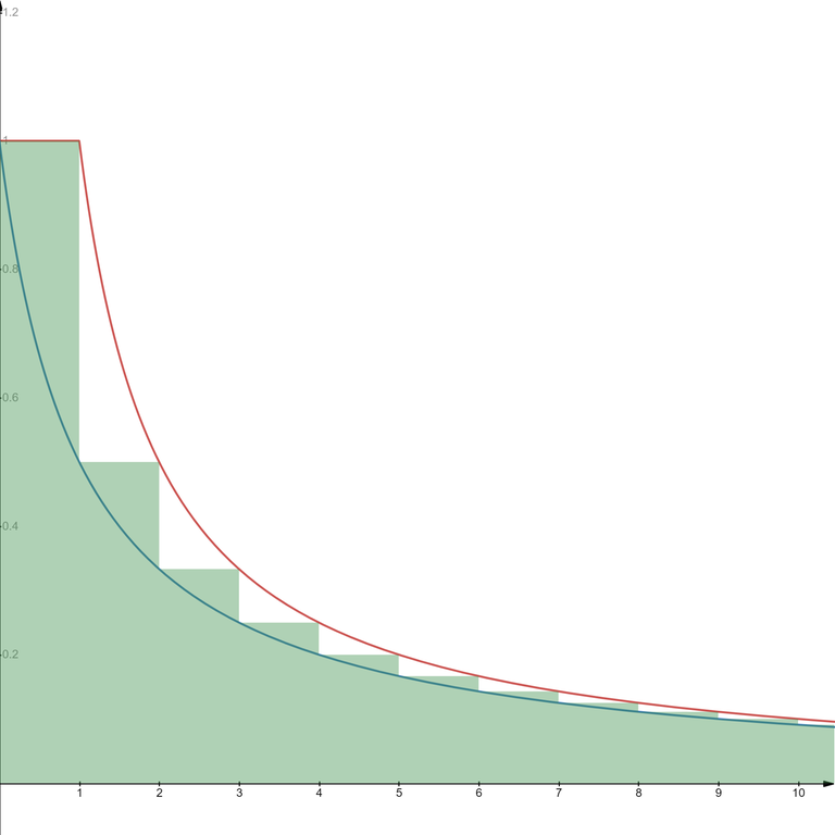
This fact is useful in calculating complexities of certain algorithms. In particular, this is common in algorithms that look like this:
1 for i in 1..n:
2     for (int k = i; k <= n; k += i):
3         # whatever
For a fixed $$$i$$$, no more than $$$\frac{n}{i}$$$ values of $$$k$$$ will be visited, so the total number of hits to line 3 will be no more than
so the complexity of this part of the algorithm is $$$O(n \log n)$$$.
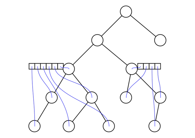
7. $$$O(n^2)$$$ complexity of certain tree DPs
Suppose you are solving a tree problem with dynamic programming. Your DP states look like this: for every vertex $$$u$$$ you have a vector $$$dp[u]$$$ and the length of this vector is at most the number of descendants of $$$u$$$. The DP is calculated like this:
 1 function calc_dp (u):
 2     for each child v of u:
 3         calc_dp(v)
 4     for each child v of u:
 5         for each child w of u other than v:
 6             for i in 0..length(dp[v])-1:
 7                 for j in in 0..length(dp[w])-1:
 8                     # calculate something
 9                     # typically based on dp[v][i] and dp[w][j]
10                     # commonly assign to dp[u][i + j]
11
12 calc_dp(root)
The complexity of this is $$$O(n^2)$$$ (this is not obvious: when I first saw it I didn't realize it was better than cubic).
8. Probabilistic treatment of number theoretic objects
This trick is not mathematically rigorous. Still, it is useful and somewhat reliable for use in heuristic/"proof by AC” algorithms. The idea is to pretend that things in number theory are just random. Examples:
- Pretend the prime numbers are a random subset of the natural numbers, where a number $$$n \ge 2$$$ is prime with probability $$$\frac1{\log n}$$$.
- Let $$$p > 2$$$ be prime. Pretend that the quadratic residues modulo $$$p$$$ are a random subset of $$$1, \ldots, p-1$$$, where a number is a quadratic residue with probability $$$\frac12$$$.
A quadratic residue modulo $$$p$$$ is any number $$$a$$$ that can be represented as a square modulo $$$p$$$; that is, there exists some $$$b$$$ such that $$$a \equiv b^2 \pmod{p}$$$.
The actual, mathematically true facts:
- There are $$$\Theta \left( \frac{n}{\log n} \right)$$$ primes up to $$$n$$$.
- Given a prime $$$p > 2$$$, there are exactly $$$\frac{p - 1}{2}$$$ quadratic residues.
Many actual, practical number theoretic algorithms use these ideas. For example, Pollard's rho algorithm works by pretending that a certain sequence $$$x_i \equiv x^2_{i - 1} + 1 \pmod{n}$$$ is a sequence of random numbers. Even the famous Goldbach's conjecture can be seen as a variation of this trick. On a lighter note, this is also why it is possible to find prime numbers like this:
Prime numbers are plentiful, so it's easy to create such pictures by taking a base picture and changing positions randomly.
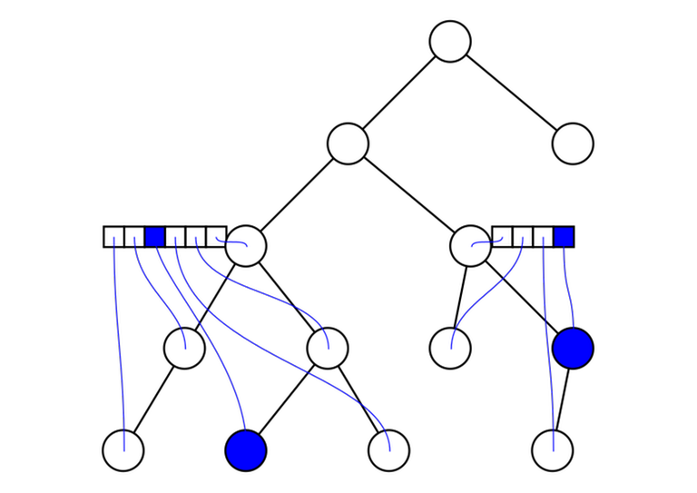
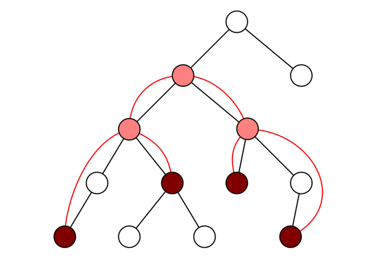
9. LCAs induced by a subset of vertices
Given a tree and a subset of vertices $$$v_1, v_2, \ldots, v_m$$$. Let's reorder them in the (preorder) DFS order. For any $$$i$$$ and $$$j$$$ with $$$v_i \ne v_j$$$, $$$\mathrm{lca}(v_i, v_j) = \mathrm{lca}(v_k, v_{k + 1})$$$ for some $$$k$$$. In other words: the lowest common ancestor of any two vertices in the array can be represented as the lowest common ancestor of two adjacent vertices.
10. Erdős–Szekeres theorem
Consider a permutation $$$p$$$ with length $$$n$$$. At least one of the following is true:
- There exists an increasing subsequence with length $$$\sqrt{n}$$$.
- There exists a decreasing subsequence with length $$$\sqrt{n}$$$.
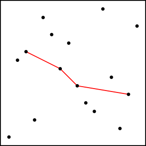
On this image we can see one possible decreasing subsequence of length 4 in a permutation of length 16. There are many options, some longer than 4.
Alternatively, we may phrase this as a fact about the longest increasing and decreasing sequences.
Thank you for reading! 10 is a good number, I think I've reached a good length of a blog post for now.

