Блог пользователя pajenegod

Автор pajenegod, история, 2 месяца назад, По-английски

Yesterday, investigating Strange TLE by cin using GNU C++20 (64), I found an easy and reproducable way to trigger a slowdown bug that I believe has been plaguing Codeforces for some time now. So I'm making this blog to raise awarness of it. MikeMirzayanov, please take a look at this!

Here is how to trigger the slowness bug:

  1. Take any problem with a relatively large input on Codeforces ($$$2 \cdot 10^5$$$ ints is enough).
  2. Take a random AC C++ submission that uses std::cin.
  3. Add the line vector<vector<int>> TLE(40000, vector<int>(7)); somewhere in global space.
  4. Submit using either C++20(64 bit) or C++17(64 bit).
  5. ???
  6. TLE

For example take tourist's solution to problem 1936-D - Bitwise Paradox. With the vector of death added to the code, it gets TLE on TC5 (taking $$$> 5$$$ s). While without the deadly vector, the submission takes 155 ms on TC5.

Here is a stand alone example with the slowdown (credit to kostia244). It runs 100 times slower with the vector of death.

#include<bits/stdc++.h>
using namespace std;

vector<vector<int>> TLE(40000, vector<int>(7));

int main() {
    string s;
    for(int i = 0; i < 17; i++) s += to_string(i) + " ";
    
    for (int j = 0; j < 60000; ++j) {
        istringstream ss(s);
        int x;
        while (ss >> x);
    }
}
What is causing this?
Other ways to trigger the slowdown bug
Other blogs on this topic

Полный текст и комментарии »

  • Проголосовать: нравится
  • +658
  • Проголосовать: не нравится

Автор pajenegod, история, 3 месяца назад, По-английски

Hi Codeforces!

Today I want to tell you about a really cool and relatively unknown technique that is reminiscent of Centroid decomposition, but at the same time is also completely different.

The most common and well known decomposition tree algorithm out there is the centroid decomposition algorithm (running in $$$O(n \log n)$$$). It is a standard algorithm that is commonly used to solve tons of different kind of divide and conquer problems on trees. However, it turns out that there exists another closely related decomposition tree algorithm, that is in a sense optimal, and can be implemented to run in $$$O(n)$$$ time in around $$$30$$$ lines of code. I have chosen to call it the Shallowest Decomposition Tree. This blog will be all about the shallowest decomposition tree. Something I want to remark on before we start is that I did not invent this. However, very few people know about it. So I decided to make this blog in order to teach people about this super cool and relatively unknown technique!

I believe that part of the reason for why the shallowest decomposition tree is almost never used in practice is because no one has published a simple to use implementation of it. My contribution here is that I've come up with a slick and efficient implementation that constructs the decomposition in linear time. I've implemented it both in Python and C++.

Shallowest Decomposition Tree:

C++ Implementation
Python implementation (with recursion)
Python implementation (without recursion)

And for comparison, here are also a couple of centroid decomposition tree implementations using the same interface.

Centroid Decomposition Tree:

C++ implementation
Python implementation

1. Motivation / Background

Take a look at the following problem

Treasure Hunt on a Tree (interactive)

1.1. What exactly is a "decomposition tree"?

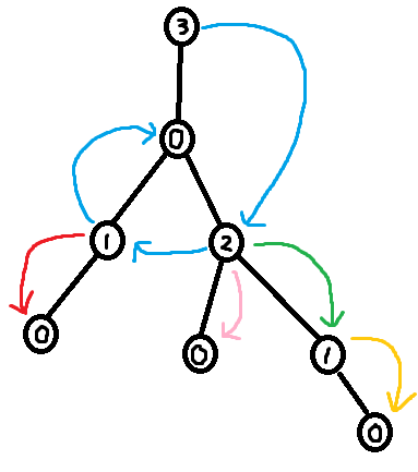
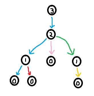
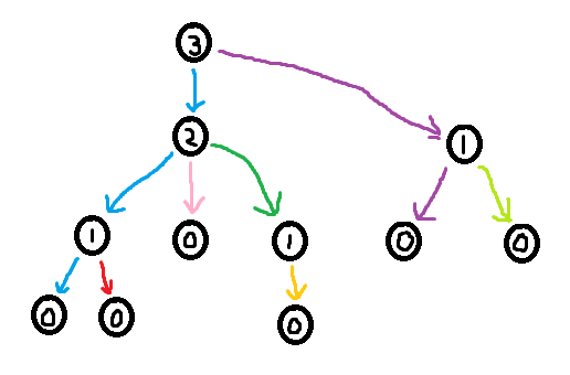
Think about how one could visualize a deterministic strategy in the treasure hunt game. One natural way to do it is to create a new tree where the root of this new tree is the first node you guess. The children of this root are all the possible 2nd guesses (which depend on the result of the first guess). Then do the same for 3rd guesses, 4th guesses, etc. I am going to refer to this resulting tree as a decomposition tree of the original tree. Note that the goal of minimizing the number of guesses is equivalent to constructing the shallowest possible decomposition tree.

1.2. The centroid guessing strategy

A natural strategy for the treasure hunt game is to guess the centroid of the tree. The definition of a centroid is a node, such that if removed from the tree, would split the tree into subtrees such that all subtrees have a size $$$\leq n/2$$$. Note that trees always have at least one centroid, and can have up to a maximum of 2 centroids.

In practice, a common way to find a centroid is to start at some arbitrary node $$$u$$$, try splitting the tree at $$$u$$$, and find the largest subtree from the split. If the size of the largest subtree is $$$> n/2$$$, then you move $$$u$$$ in the direction of that subtree. If the size of the largest subtree $$$\leq n/2$$$, then $$$u$$$ is a centroid, and so you have found a centroid.

By repeatedly guessing centroids in the treasure hunt problem, the set of nodes the treasure could be hidden at is guaranteed to decrease by at least a factor of $$$2$$$ for each guess. This will lead to having to do at most $$$\log_2(n)$$$ guesses in worst case. However, it turns out there examples of trees where this centroid guessing strategy is sub-optimal.

1.2.1. Examples of trees where the centroid guessing strategy is not optimal

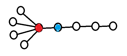
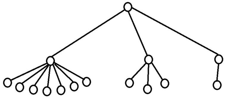
Small example where centroid decomposition is a factor 4/3 from optimal
Construction where centroid decomposition is a factor O(log n) from optimal

1.3. The center guessing strategy

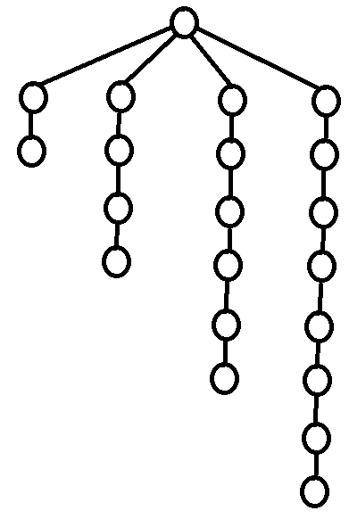
Another natural strategy for the treasure hunt game is to guess the center of the tree, i.e. the least eccentric vertex (the "middle node" of the diameter). This turns out to be a fairly bad strategy, as can be seen in the following counter example (credit to dorijanlendvaj for this example).

Construction where center decomposition is a factor O(sqrt(n)/log(n)) from optimal

2. Shallowest decomposition tree

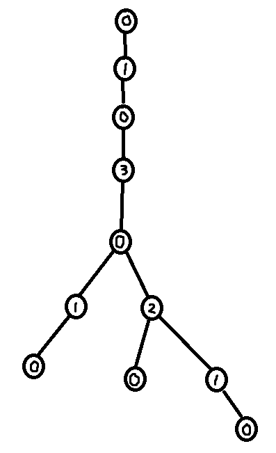
Now we are finally at the point where we can talk about how to find the optimal (the shallowest) decomposition tree. The key to finding the shallowest decomposition tree turns out to be a greedy solution of a certain "Labeling Problem" 321C - Ciel the Commander.

The Labeling Problem

It turns out that this labeling problem can be solved optimally by labeling greedily.

Greedy labeling

In the next section, we will prove that greedy labeling is in fact optimal, and we will also show how to construct it in linear time.

Something that is very important to note is that it is possible to extract a decomposition tree from a labeling. The highest labeled node must have a unique label (because of constraint 2). So start by picking the highest labeled node as the root for the decomposition. Then remove that node and recurse. This will lead to a decomposition tree of depth $$$\leq$$$ largest label.

Also note that given a decomposition tree it is possible to create a labeling. One way to do this is to label the nodes by their height in the decomposition tree. This will make it so the largest label used $$$=$$$ depth of the decomposition tree.

The take away from this discussion is that optimally solving the labeling problem is equivalent to finding an optimal deterministic strategy in the treasure hunt game, since a solution to the labeling problem can be made into a deterministic strategy for the treasure hunt game, and vice versa. So our (optimal) greedy labeling corresponds to an (optimal) deterministic guessing strategy in the treasure hunt game.

3. Analysis of greedy labeling

Let us first define the notion of forbidden labels. Given a rooted tree, a labeling of the tree, and a node $$$u$$$ in the tree, define forbidden(u) as the bitmask describing all labels that cannot be put on $$$u$$$ considering the descendants of $$$u$$$. I.e. bit $$$i$$$ of forbidden(u) is $$$1$$$ if and only if labeling node $$$u$$$ with label $$$i$$$ would cause a contradiction with the labels of the descendants of $$$u$$$.

Note that in the case of the greedy labeling, the label of $$$u$$$ corresponds to the least significant set bit of forbidden(u) + 1, or equivalently it is the number of trailing zeroes of forbidden(u) + 1.

3.1 A O(n) DP-algorithm for greedy labeling.

In the case of the greedy labeling, it is possible to make a DP-formula for forbidden(u). There are 3 cases:

Case 1. Node $$$u$$$ has no children. In this case forbidden(u) = 0.

Case 2. Node $$$u$$$ has exactly one child $$$v$$$. In this case forbidden(u) = forbidden(v) + 1.

Case 3. Node $$$u$$$ has multiple children, $$$v_1$$$, ..., $$$v_m$$$. In this case bit $$$i$$$ is set in forbidden(u) if either

  • bit $$$i$$$ is set in at least one of forbidden(v_1) + 1, ..., forbidden(v_m) + 1.

  • or there exists $$$j > i$$$ such that bit $$$j$$$ is set in at least two of forbidden(v_1) + 1, ..., forbidden(v_m) + 1.

This gives us a simple O(n) implementation of the greedy labeling algorithm.

# Count trailing zeros
# Or equivalently, index of lowest set bit
def ctz(x): 
    return (x & -x).bit_length() - 1

forbidden = [0] * n
def dfs(u, p):
    forbidden_once = forbidden_twice = 0
    for v in graph[u]:
        if v != p:
            dfs(v, u)
            forbidden_by_v = forbidden[v] + 1
            forbidden_twice |= forbidden_once & forbidden_by_v
            forbidden_once |= forbidden_by_v
    forbidden[u] = forbidden_once | (2**forbidden_twice.bit_length() - 1)
dfs(root, -1)
labels = [ctz(forbidden[u] + 1) for u in range(n)]

Remark: It is not actually obvious why this algorithm runs in linear time since this algorithm could in theory be using big integers. But as we will see in the next section, Section 3.2, greedy labeling is optimal. So by comparing the greedy labeling to centroid labeling, we know that the largest forbidden label for the greedy labeling is upper bounded by $$$\log_2(n)$$$. So this DP-algorithm does not use any big integers, and is therefore just a standard dfs algorithm which runs in linear time.

3.2 Greedy labeling is optimal

Lemma: Given a rooted tree (rooted at some node $$$r$$$). Out of all possibly labelings of this rooted tree, the greedy labeling (with root $$$r$$$) minimizes forbidden(r).

Note that minimizing forbidden(r) is effectively the same thing as minimizing the largest label used in the labeling. So it follows from this claim that the greedy algorithm uses the fewest number of distinct labels out of any valid labeling.

Proof of Lemma

3.3. Adv. Constructing the shallowest decomposition tree in linear time

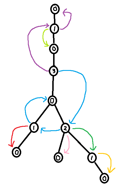
As seen in section 3.2, it is easy to construct the greedy labeling in linear time. However, it is far more tricky to construct the shallowest decomposition tree in $$$O(n)$$$ time. The way we will do it is by making use of chains. Before we formally define what a chain is, take a look at the following examples.

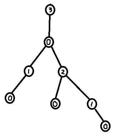
Basic example
More general example

So formally,

Definition of the chains of a rooted labeled tree

Using the forbidden variable, it is possible to identify these chains. If $$$v$$$ is a child of $$$u$$$, then set of labels in forbidden(v) + 1 which are smaller than $$$u$$$'s label corresponds to a (Case 1) chain. Furthermore, the set of labels in forbidden(root) + 1 corresponds to the (Case 2) chain. So we can easily identify the sets of labels making up the chains. However, what we need in order to build the decomposition tree is to find the set of nodes that make up the chains.

The last trick we need is to use $$$O(\log n)$$$ stacks (one stack for each label). To extract the shallowest decomposition tree. Do a DFS over the greedily labeled tree. When we first visit a node, append that node into its corresponding stack. Furthermore, during the dfs, whenever we identify the labels of a chain, we can pop the corresponding stacks in order to find the nodes making up that chain. Then add the chain edges to the decomposition tree. I've called this popping procedure extract_chain in the code below.

Extraction of decomposition tree using chains implemented in Python

With this, the linear time algorithm for the shallowest decomposition tree is finally complete! However, it is still possible to make some slight improvements. The main improvement would be to greedy label and build the decomposition tree at the same time in a single dfs, instead of using two dfs's. This is what I've chosen to do in my Python and C++ implementations found at the top of this blog. Another possible improvement is to have a variable for forbidden[u] + 1 instead of forbidden[u] itself. Because of comprehensibility, I've chosen not to do this. But it would definitely help if you'd want to codegolf it. The final possible improvement is to switch from using a recursive dfs to manually doing the dfs using a stack. This improvement is important for languages that don't handle recursion well, like Python.

4. Benchmarks

To my knowledge, every problem that can be solved with centroid decomposition can be solved with shallowest decomposition tree too, and you can freely switch between them. So here are a couple of comparisons between the two decompositions.

321C - Ciel the Commander
Centroid (Python) TLE 1.34 s / 1 s | Shallowest (Python) 0.72 s | Centroid (C++) 0.28 s | Shallowest (C++) 0.16 s
914E - Palindromes in a Tree
Centroid (Python) TLE 4.2 s / 4 s | Shallowest (Python) 3.75 s | Centroid (C++) 1.67 s | Shallowest (C++) 1.53 s

321C - Ciel the Commander is a good example of a problem where most of the time is spent building the decomposition tree. Here we can see a fairly significant boost from using the Shallowest Decomposition Tree compared to using Centroid Decomposition, especially if we take away the time spent on IO. 914E - Palindromes in a Tree is a good example of a problem where building the decomposition tree only takes up a small portion of the total time. For this reason, we only see a small performance gain from using the Shallowest Decomposition Tree.

Remark: There are definitely faster solutions to 321C - Ciel the Commander out there. For example, you could solve the problem just by outputting a greedy labeling without ever constructing any kind of decomposition tree. But the reason I'm using this problem as a benchmark is to compare the time used to construct the shallowest decomposition tree vs the centroid decomposition tree.

5. Mentions and final remarks

A big thanks Devil for introducing the shallowest decomposition tree to me. Also a big thanks to everyone that has discussed the shallowest decomposition tree with me over at the AC server. qmk magnus.hegdahl nor gamegame Savior-of-Cross meooow brunovsky PurpleCrayon.

One final thing I want to mention is that I know of two competitive programming problems that are intended to be solved specifically using the shallowest decomposition tree. Chronologically, the first problem is Cavern from POI. From what I understand, they were the first to come up with the idea. Many years later, atcoder independently came up with Uninity.

There has also been a much more recent problem 1444E - Finding the Vertex, which is a treasure hunt game on a tree, where you are allowed to guess edges instead of nodes. The solution isn't exactly the shallowest decomposition tree, but the method used to solve it is closely related to the shallowest decomposition tree. I challenge anyone that think they've mastered shallowest decomposition tree to solve it. If you need help on it, then take a look at my submission 242905032.

Полный текст и комментарии »

  • Проголосовать: нравится
  • +403
  • Проголосовать: не нравится

Автор pajenegod, история, 4 месяца назад, По-английски

Hi Codeforces!

Have you ever had this issue before?

If yes, then you have come to the right place! This is a blog about my super easy to use template for (reroot) DP on trees. I really believe that this template is kind of revolutionary for solving reroot DP problems. I've implemented it both in Python and in C++ (the template supports Python2, Python3 and >= C++14). Using this template, you will be able to easily solve > 2000 rated reroot problems in a couple of minutes, with a couple of lines of code.

A big thanks goes out to everyone that has helped me by giving feedback on blog and/or discussing reroot with me, nor, meooow, qmk, demoralizer, jeroenodb, ffao. And especially a huge thanks goes to nor for helping out making the C++ version of the template.

1. Introduction / Motivation

As an example, consider this problem: 1324F - Maximum White Subtree. The single thing that makes this problem difficult is that you need for every node $$$u$$$ find the maximum white subtree containing $$$u$$$. Had this problem only asked to find the answer for a specific node $$$u$$$, then a simple dfs solution would have worked.

Simple dfs solution

But 1324F - Maximum White Subtree requires you to find the answer for every node. This forces you to use a technique called rerooting. Long story short, it is a mess to code. Maybe you could argue that for this specific problem it isn't all that bad. But it is definitely not as easy to code as the dfs solution above.

What if I told you that it is possible to take the logic from the dfs function above, put it inside of a "black box", and get the answer for all $$$u$$$ in $$$O(n \log n)$$$ time? Well it is, and that is what this blog is all about =)

In order to extract the logic from the simple dfs solution, let us first create a generic template for DP on trees and implement the simple dfs solution using its interface. Note that the following code contain the exact same logic as the simple dfs solution above. It solves the problem for a specific node $$$u$$$.

Simple dfs solution (using treeDP template)

Now, all that remains to solve the full problem is to switch out the treeDP function with the ultimate reroot template. The template returns the output of treeDP for every node $$$u$$$, in $$$O(n \log n)$$$ time! It is just that easy. 240150867

Solution to problem F using the ultimate reroot template

The takeaway from this is example is that the reroot template makes it almost trivial to solve complicated reroot problems. For example, suppose we modify 1324F - Maximum White Subtree such that both nodes and edges have colors. Normally this modification would be complicated and would require an entire overhaul of the solution. However, with the ultimate reroot template, the solution is simply:

Solution to problem F if both edges and nodes are colored

2. Collection of reroot problems and solutions

Here is a collection of reroot problems on Codeforces, together with some short and simple solutions in both Python and C++ using the rerooter template. These are nice problems to practice on if you want to try out using this template. The difficulty rating ranges between 1700 and 2600. I've also put together a GYM contest with all of the problems: Collection of Reroot DP problems (difficulty rating 1700 to 2600).

(1700 rating) 219D - Choosing Capital for Treeland
Python solution, C++ solution
(2300 rating) 543D - Road Improvement
Python solution, C++ solution
(2200 rating) 592D - Super M
Python solution, C++ solution
(2600 rating) 627D - Preorder Test
Python solution, C++ solution
(2100 rating) 852E - Casinos and travel
Python solution, C++ solution
(2300 rating) 960E - Alternating Tree
Python solution, C++ solution
Or alternatively using "edge DP":
Python solution, C++ solution
(1900 rating) 1092F - Tree with Maximum Cost
Python solution, C++ solution
(2200 rating) 1156D - 0-1-Tree
Python solution, C++ solution
(2400 rating) 1182D - Complete Mirror
Python solution, C++ solution
(2100 rating) 1187E - Tree Painting
Python solution, C++ solution
(2000 rating) 1294F - Three Paths on a Tree
Python solution, C++ solution
(1800 rating) 1324F - Maximum White Subtree
Python solution, C++ solution
(2500 rating) 1498F - Christmas Game
Python solution, C++ solution
(2400 rating) 1626E - Black and White Tree
Python solution, C++ solution
(2500 rating) 1691F - K-Set Tree
Python solution, C++ solution
(2400 rating) 1794E - Labeling the Tree with Distances
Python solution, C++ solution
(2500 rating) 1796E - Colored Subgraphs
Python solution, C++ solution
(1700 rating) 1881F - Minimum Maximum Distance
Python solution, C++ solution
104008G - Group Homework
Python solution, C++ solution
104665H - Alice Learns Eertree!
Python solution, C++ solution

3. Understanding the rerooter black box

The following is the black box rerooter implemented naively:

Template (naive O(n^2) version)

rerooter outputs three variables.

  1. rootDP is a list, where rootDP[node] = dfs(node).
  2. forwardDP is a list of lists, where forwardDP[node][eind] = dfs(nei, node), where nei = graph[node][eind].
  3. reverseDP is a list of lists, where reverseDP[node][eind] = dfs(node, nei), where nei = graph[node][eind].

If you don't understand the definitions of rootDP/forwardDP/reverseDP, then I recommend reading the naive $$$O(n^2)$$$ implementation of rerooter. It should be fairly self explanatory.

The rest of this blog is about the techniques of how to make rerooter run in $$$O(n \log n)$$$. So if you just want to use rerooter as a black box, then you don't have to read or understand the rest of this blog.

One last remark. If you've ever done rerooting before, you might recall that rerooting usually runs in $$$O(n)$$$ time. So why does this template run in $$$O(n \log n)$$$? The reason for this is that I restrict myself to use the combine function in a left folding procedure, e.g. combine(combine(combine(nodeDP, neiDP1), neiDP2), neiDP3). My template is not allowed to do for example combine(nodeDP, combine(neiDP1, combine(neiDP2, neiDP3))). While this limitation makes the template run slower, $$$O(n \log n)$$$ instead of $$$O(n)$$$, it also makes it a lot easier to use the template. If you still think that the $$$O(n)$$$ version is superior, then I don't think you've understood how nice and general the $$$O(n \log n)$$$ version truly is.

4. Rerooting and exclusivity

The general idea behind rerooting is that we first compute the DP as normal for some arbitrary node as the root (I use node = 0 for this). After we have done this we can "move" the root of the tree by updating the DP value of the old root and the DP value of a neighbour to the old root. That neighbour then becomes the new root.

Let $$$u$$$ denote the current root, and let $$$v$$$ denote the neighbour of $$$u$$$ that we want to move the root to. At this point, we already know the value of dfs(v, u) since $$$u$$$ is the current root. But in order to be able to move the root from $$$u$$$ to $$$v$$$, we need to find the new DP value of $$$u$$$, i.e. dfs(u, v).

If we think about this in terms of forwardDP and reverseDP, then we currently know forwardDP[u], and our goal is to compute reverseDP[u]. This can be done naively in $$$O(\text{deg}(u)^2)$$$ time with a couple of for loops by calling combine $$$O(\text{deg}(u)^2)$$$ times, and then calling finalize $$$O(\text{deg}(u))$$$ times.

The bottle neck here are the $$$O(\text{deg}(u)^2)$$$ calls to combine. So for now, let us separate out the part of the code that calls combine from the rest of the code into a function called exclusive. The goal of the next section will then be to speed up the naively implemented exclusive function to run in $$$O(\text{deg}(u) \text{log} (\text{deg}(u)))$$$ time.

Rerooting using exclusivity (O(sum deg^2) version)

5. The exclusive segment tree

We are almost done implementing the fast reroot template. The only operation left to speed up is the function exclusive. Currently it runs in $$$O(\sum \text{deg}^2)$$$ time. The trick to make exclusive run in $$$O(\sum \text{deg} \log{(\text{deg})})$$$ time is to create something similar to a segment tree.

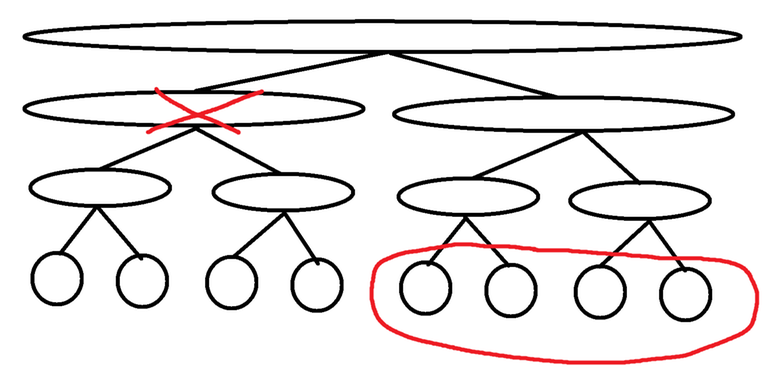
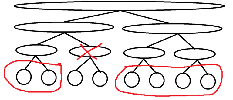
Suppose you have a segment tree where each node in the segment tree accumulates all of the values outside of its interval. The leaves of such a segment tree can then be used as the output of exclusive. I call this data structure the exclusive segment tree.

Example: Exclusive segment tree of size n = 8

The exclusive segment tree is naturally built from top to bottom, taking $$$O(n \log n)$$$ time. Here is an implementation of rerooter using the exclusive segment tree:

Rerooting using exclusivity (O(sum deg log(deg)) version)

This algorithm runs in $$$O(\sum \text{deg} \log{(\text{deg})})$$$, so we are essentially done. However, this implementation uses recursive DFS which especially for Python is a huge drawback. Recursion in Python is both relatively slow and increadibly memory hungry. So for a far more practical version, I've also implemented this same algorithm using a BFS instead of a DFS. This gives us the final version of the ultimate rerooter template!

Rerooting using exclusivity (O(sum deg log(deg)) version with BFS)

Полный текст и комментарии »

  • Проголосовать: нравится
  • +489
  • Проголосовать: не нравится

Автор pajenegod, история, 9 месяцев назад, По-английски

I don't think blogs like this one should be normal on Codeforces.

I know that sometimes comments can be frustrating. Sometimes it is the commenters fault, and sometimes it is the community's fault for upvoting mean spirited comments. I understand that in some cases, the criticism the commenter receives is fair and well-deserved.

But there is a fine line between criticism, saying that you didn't like the comment, and hanging out a comment on the front page and letting everyone attack it. The former two are acceptable (and sometimes even needed, because commenter have to improve and learn from their mistakes); the latter one, in my opinion, should not be acceptable.

I think that blogs discussing toxicity on codeforces are a good thing, but singling out a comment made by some kid onto the front page of Codeforces is a very inconsiderate and irresponsible thing to do.

Полный текст и комментарии »

  • Проголосовать: нравится
  • +391
  • Проголосовать: не нравится

Автор pajenegod, история, 10 месяцев назад, По-английски

Hi Codeforces!

I have something exciting to tell you guys about today! I have recently come up with a really neat and simple recursive algorithm for multiplying polynomials in $$$O(n \log n)$$$ time. It is so neat and simple that I think it might possibly revolutionize the way that fast polynomial multiplication is taught and coded. You don't need to know anything about FFT to understand and implement this algorithm.

Big thanks to nor, c1729 and Spheniscine for discussing the contents of the blog with me and comming up with ideas for how to improve the blog =).

I've split this blog up into two parts. The first part is intended for anyone to be able to read and understand. The second part is advanced and goes into a ton of interesting ideas and concepts related to this algorithm.

Prerequisite: Polynomial quotient and remainder, see Wiki article and this Stackexchange example.

Task:

Given two polynomials $$$P$$$ and $$$Q$$$, an integer $$$n$$$ and a non-zero complex number $$$c$$$, where degree $$$P < n$$$ and degree $$$Q < n$$$. Your task is to calculate the polynomial $$$P(x) \, Q(x) \% (x^n - c)$$$ in $$$O(n \log n)$$$ time. You may assume that $$$n$$$ is a power of two.

Solution:

We can create a divide and conquer algorithm for $$$P(x) \, Q(x) \% (x^n - c)$$$ based on the difference of squares formula. Assuming $$$n$$$ is even, then $$$(x^n - c) = (x^{n/2} - \sqrt{c}) (x^{n/2} + \sqrt{c})$$$. The idea behind the algorithm is to calculate $$$P(x) \, Q(x) \% (x^{n/2} - \sqrt{c})$$$ and $$$P(x) \, Q(x) \% (x^{n/2} + \sqrt{c})$$$ using 2 recursive calls, and then use that result to calculate $$$P(x) \, Q(x) \% (x^n - c)$$$.

So how do we actually calculate $$$P(x) \, Q(x) \% (x^n - c)$$$ using $$$P(x) \, Q(x) \% (x^{n/2} - \sqrt{c})$$$ and $$$P(x) \, Q(x) \% (x^{n/2} + \sqrt{c})$$$?

Well, we can use the following formula:

$$$ \begin{aligned} A(x) \% (x^n - c) = &\frac{1}{2} \left(1 + \frac{x^{n/2}}{\sqrt{c}}\right) \left(A(x) \% (x^{n/2} - \sqrt{c})\right) \, + \\ &\frac{1}{2} \left(1 - \frac{x^{n/2}}{\sqrt{c}}\right) \left(A(x) \% (x^{n/2} + \sqrt{c})\right). \end{aligned} $$$
Proof of the formula

This formula is very useful. If we substitute $$$A(x)$$$ by $$$P(x) Q(x)$$$, then the formula tells us how to calculate $$$P(x) \, Q(x) \% (x^n - c)$$$ using $$$P(x) \, Q(x) \% (x^{n/2} - \sqrt{c})$$$ and $$$P(x) \, Q(x) \% (x^{n/2} + \sqrt{c})$$$ in linear time. With this we have the recipie for implementing a $$$O(n \log n)$$$ divide and conquer algorithm:

Input:

  • Integer $$$n$$$ (power of 2),
  • Non-zero complex number $$$c$$$,
  • Two polynomials $$$P(x) \% (x^n - c)$$$ and $$$Q(x) \% (x^n - c)$$$.

Output:

  • The polynomial $$$P(x) \, Q(x) \% (x^n - c)$$$.

Algorithm:

Step 1. (Base case) If $$$n = 1$$$, then return $$$P(0) \cdot Q(0)$$$. Otherwise:

Step 2. Starting from $$$P(x) \% (x^n - c)$$$ and $$$Q(x) \% (x^n - c)$$$, in $$$O(n)$$$ time calculate

$$$ \begin{align} & P(x) \% (x^{n/2} - \sqrt{c}), \\ & Q(x) \% (x^{n/2} - \sqrt{c}), \\ & P(x) \% (x^{n/2} + \sqrt{c}) \text{ and} \\ & Q(x) \% (x^{n/2} + \sqrt{c}). \end{align} $$$

Step 3. Make two recursive calls to calculate $$$P(x) \, Q(x) \% (x^{n/2} - \sqrt{c})$$$ and $$$P(x) \, Q(x) \% (x^{n/2} + \sqrt{c})$$$.

Step 4. Using the formula, calculate $$$P(x) \, Q(x) \% (x^n - c)$$$ in $$$O(n)$$$ time. Return the result.

Here is a Python implementation following this recipie:

Python solution to the task

One final thing that I want to mention before going into the advanced section is that this algorithm can also be used to do fast unmodded polynomial multiplication, i.e. given polynomials $$$P(x)$$$ and $$$Q(x)$$$ calculate $$$P(x) \, Q(x)$$$. The trick is simply to pick $$$n$$$ large enough such that $$$P(x) \, Q(x) = P(x) \, Q(x) \% (x^n - c)$$$, and then use the exact same algorithm as before. $$$c$$$ can be arbitrarily picked (any non-zero complex number works).

Python implementation for general Fast polynomial multiplication

If you want to try out implementing this algorithm yourself, then here is a very simple problem to test out your implementation on: SPOJ:POLYMUL.

(Advanced) Speeding up the algorithm

This section will be about tricks that can be used to speed up the algorithm. The first two tricks will speed up the algorithm by a factor of 2 each. The last trick is advanced, and it has the potential to both speed up the algorithm and also make it more numerically stable.

$n$ doesn't actually need to be a power of 2
Imaginary-cyclic convolution
Calculating fast_polymult_mod(P, Q, n, c) using using fast_polymult_mod(P, Q, n, 1) (reweight technique)

(Advanced) -is-this-fft-?

This algorithm is actually FFT in disguise. But it is also different compared to any other FFT algorithm that I've seen in the past (for example the Cooley–Tukey FFT algorithm).

Using this algorithm to calculate FFT
This algorithm is not the same algorithm as Cooley–Tukey
FFT implementation in Python based on this algorithm
FFT implementation in C++ based on this algorithm

(Advanced) Connection between this algorithm and NTT

Just like how there is FFT and NTT, there are two variants of this algorithm too. One using complex floating point numbers, and the other using modulo a prime (or more generally modulo an odd composite number).

Using modulo integers instead of complex numbers
Calculating fast_polymult_mod(P, Q, n, c) using fast_polymult_mod(P, Q, 2*n, 1)
This algorithm works to some degree even for bad NTT primes
NTT implementation in Python based on this algorithm
NTT implementation in C++ based on this algorithm
Blazingly fast NTT C++ implementation

(Advanced) Shorter implementations ("Codegolfed version")

It is possible to make really short but slightly less natural implementations of this algorithm. Originally I was thinking of using this shorter version in the blog, but in the end I didn't do it. So here they are. If you want a short implemention of this algorithm to use in practice, then I would recommend taking one of these implementations and porting it to C++.

Short Python implementation without any speedup tricks
Short Python implementation supporting odd and even $n$ (making it up to 2 times faster)
Short Python implementation supporting odd and even $n$ and imaginary cyclic convolution (making it up to 4 times faster)

Полный текст и комментарии »

  • Проголосовать: нравится
  • +349
  • Проголосовать: не нравится

Автор pajenegod, история, 13 месяцев назад, По-английски

Take a look at this C++ submission 199864568:

#import <bits/stdc++.h>
using namespace std;
int main()
{
    int a; 
    cin >> a; 
    cout << ((a%2==0 && a>2) ? "YES" : "NO");
}

Don't see it?
Spoilers

Полный текст и комментарии »

  • Проголосовать: нравится
  • +312
  • Проголосовать: не нравится

Автор pajenegod, история, 19 месяцев назад, По-английски

I recently had a very interesting idea for how to greatly speed up convolution (a.k.a. polynomial multiplication).

def convolution(A, B):
  C = [0] * (len(A) + len(B) - 1)
  for i in range(len(A)):
    for j in range(len(B)):
      C[i + j] += A[i] * B[j]
  return C

The standard technique for how to do convolution fast is to make use of cyclic convolution (polynomial mult mod $$$x^n - 1$$$).

def cyclic_convolution(A, B):
  n = len(A) # A and B needs to have the same size
  C = [0] * n
  for i in range(n):
    for j in range(n):
      C[(i + j) % n] += A[i] * B[j]
  return C

Cyclic convolution can be calculated in $$$O(n \log n)$$$ using FFT, which is really fast. The issue here is that in order to do convolution using cyclic convolution, we need to pad with a lot of 0s to not be affected by the wrap around. All this 0-padding feels very inefficient.

So here is my idea. What if we do polynomial multiplication mod $$$x^n - i$$$ instead of mod $$$x^n - 1$$$? Then when we get wrap around, it will be multiplied by the imaginary unit, so it wont interfere with the real part! I call this the imaginary cyclic convolution.

def imaginary_cyclic_convolution(A, B):
  n = len(A) # A and B needs to have the same size
  C = [0] * n
  for i in range(n):
    for j in range(n):
      C[(i + j) % n] += (1 if i + j < n else 1j) * A[i] * B[j]
  return C

Imaginary cyclic convolution is the perfect algorithm to use for implementing convolution. Using it, we no longer need to do copious amount of 0 padding, since the imaginary unit will take care of the wrap around. In fact, the size (the value of $$$n$$$) required is exactly half of what we would need if we had used cyclic convolution.

One question still remains, how do we implement imaginary cyclic convolution efficiently?

The trick is rather simple. Let $$$\omega = i^{\frac{1}{n}}$$$. Now note that if $$$C(\omega x) = A(\omega x) B(\omega x) \mod x^n - 1$$$ then $$$C(x) = A(x) B(x) \mod x^n - i$$$. So here is the algorithm

def imaginary_cyclic_convolution(A, B):
  n = len(A) # A and B needs to have the same size
  w = (1j)**(1/n) # n-th root of imaginary unit
  
  # Transform the polynomials A(x) -> A(wx) and B(x) -> B(wx)
  A = [A[i] * w**i for i in range(n)]
  B = [B[i] * w**i for i in range(n)]

  C = cyclic_convolution(A, B)
  
  # Transform the polynomial C(wx) -> C(x)
  C = [C[i] / w**i for i in range(n)]
  return C

Полный текст и комментарии »

  • Проголосовать: нравится
  • +157
  • Проголосовать: не нравится

Автор pajenegod, история, 20 месяцев назад, По-английски
  • Проголосовать: нравится
  • +162
  • Проголосовать: не нравится

Автор pajenegod, история, 23 месяца назад, По-английски

Hi CF! During this past weekend I was reading up on Montgomery transformation, which is a really interesting and useful technique to do fast modular multiplication. However, all of the explanations I could find online felt very unintuitive for me, so I decided to write my own blog on the subject. A big thanks to kostia244, nor, nskybytskyi and -is-this-fft- for reading this blog and giving me some feedback =).

Fast modular multiplication

Let $$$P=10^9+7$$$ and let $$$a$$$ and $$$b$$$ be two numbers in $$$[0,P)$$$. Our goal is to calculate $$$a \cdot b \, \% \, P$$$ without ever actually calling $$$\% \, P$$$. This is because calling $$$\% \, P$$$ is very costly.

If you haven't noticed that calling $$$\% \, P$$$ is really slow, then the reason you haven't noticed it is likely because the compiler automatically optimizes away the $$$\% \, P$$$ call if $$$P$$$ is known at compile time. But if $$$P$$$ is not known at compile time, then the compiler will have to call $$$\% \, P$$$, which is really really slow.

Montgomery reduction of $$$a \cdot b$$$

It turns out that the trick to calculate $$$a \cdot b \, \% \, P$$$ efficently is to calculate $$$a \cdot b \cdot 2^{-32} \, \% \, P$$$ efficiently. So the goal for this section will be to figure out how to calculate $$$a \cdot b \cdot 2^{-32} \, \% \, P$$$ efficently. $$$a \cdot b \cdot 2^{-32} \, \% \, P$$$ is called the Montgomery reduction of $$$a \cdot b$$$, denoted by $$$\text{m_reduce}(a \cdot b)$$$.

Idea (easy case)

Suppose that $$$a \cdot b$$$ just happens to be divisible by $$$2^{32}$$$. Then $$$(a \cdot b \cdot 2^{-32}) \, \% \, P = (a \cdot b) \gg 32$$$, which runs super fast!

Idea (general case)

Can we do something similar if $$$a \cdot b$$$ is not divisible by $$$2^{32}$$$? The answer is yes! The trick is to find some integer $$$m$$$ such that $$$(a \cdot b + m \cdot P)$$$ is divisible by $$$2^{32}$$$. Then $$$a \cdot b \cdot 2^{-32} \, \% \, P = (a \cdot b + m \cdot P) \cdot 2^{-32} \, \% \, P = (a \cdot b + m \cdot P) \gg 32$$$.

So how do we find such an integer $$$m$$$? We want $$$ (a \cdot b + m \cdot P) \,\%\, 2^{32} = 0$$$ so $$$m = (-a \cdot b \cdot P^{-1}) \,\%\, 2^{32}$$$. So if we precalculate $$$(-P^{-1}) \,\%\, 2^{32}$$$ then calculating $$$m$$$ can be done blazingly fast.

Montgomery transformation

Since the Montgomery reduction divides $$$a \cdot b$$$ by $$$2^{32}$$$, we would like some some way of multiplying by $$$2^{32}$$$ modulo $$$P$$$. The operation $$$x \cdot 2^{32} \, \% \, P$$$ is called the Montgomery transform of $$$x$$$, denoted by $$$\text{m_transform}(x)$$$.

The trick to implement $$$\text{m_transform}$$$ efficently is to make use of the Montgomery reduction. Note that $$$\text{m_transform}(x) = \text{m_reduce}(x \cdot (2^{64} \, \% \, P))$$$, so if we precalculate $$$2^{64} \, \% \, P$$$, then $$$\text{m_transform}$$$ also runs blazingly fast.

Montgomery multiplication

Using $$$\text{m_reduce}$$$ and $$$\text{m_transform}$$$ there are multiple different ways of calculating $$$a \cdot b \, \% \, P$$$ effectively. One way is to run $$$\text{m_transform}(\text{m_reduce}(a \cdot b))$$$. This results in two calls to $$$\text{m_reduce}$$$ per multiplication.

Another common way to do it is to always keep all integers transformed in the so called Montgomery space. If $$$a' = \text{m_transform}(a)$$$ and $$$b' = \text{m_transform}(b)$$$ then $$$\text{m_transform}(a \cdot b \, \% \, P) = \text{m_reduce}(a' \cdot b')$$$. This effectively results in one call to $$$\text{m_reduce}$$$ per multiplication, however you now have to pay to move integers in to and out of the Montgomery space.

Example implementation

Here is a Python 3.8 implementation of Montgomery multiplication. This implementation is just meant to serve as a basic example. Implement it in C++ if you want it to run fast.

P = 10**9 + 7
r = 2**32
r2 = r * r % P
Pinv = pow(-P, -1, r) # (-P^-1) % r

def m_reduce(ab):
  m = ab * Pinv % r
  return (ab + m * P) // r

def m_transform(a):
  return m_reduce(a * r2)

# Example of how to use it
a = 123456789
b = 35
a_prim = m_transform(a) # mult a by 2^32
b_prim = m_transform(b) # mult b by 2^32
prod_prim = m_reduce(a_prim * b_prim) # divide a' * b' by 2^32
prod = m_reduce(prod_prim) # divide prod' by 2^32
print('%d * %d %% %d = %d' % (a, b, P, prod)) # prints 123456789 * 35 % 1000000007 = 320987587

Final remarks

One important issue that I've so far swept under the rug is that the output of m_reduce is actually in $$$[0, 2 P)$$$ and not $$$[0, P)$$$. I just want end by discussing this issue. I can see two ways of handling this:

  • Alternative 1. You can force $$$\text{m_reduce}(a \cdot b)$$$ to be in $$$[0, P)$$$ for $$$a$$$ and $$$b$$$ in $$$[0, P)$$$ by adding an if-stament to the output of m_reduce. This will work for any odd integer $$$P < 2^{31}$$$.
Fixed implementation of m_reduce
  • Alternative 2. Assuming $$$P$$$ is an odd integer $$$< 2^{30}$$$ then if $$$a$$$ and $$$b$$$ $$$\in [0, 2 P)$$$ you can show that the output of $$$\text{m_reduce}(a \cdot b)$$$ is also in $$$[0,2 P)$$$. So if you are fine working with $$$[0, 2 P) \vphantom]$$$ everywhere then you don't need any if-statements. Nyaan's github has a nice C++ implementation of Montgomery multiplication using this style of implementation.

Полный текст и комментарии »

  • Проголосовать: нравится
  • +92
  • Проголосовать: не нравится

Автор pajenegod, история, 3 года назад, По-английски

I've always liked using Python (PyPy) for solving problems in competitive programming. And most problems are very doable, even in Python. What I've found is that the most difficult problems to solve in Python are those requiring 64 bit integers.

The reason why 64 bit integers are problematic is because CF runs Windows, and PyPy only supports 32 bit on Windows. So whenever a problem involves integers that cannot fit inside of a signed 32 bit int, PyPy switches to big integers (which runs insanely slow, sometimes a factor of 20 times slower).

What I currently have to do to get around big integers

However with the latest PyPy version (version 7.3.4) PyPy has finally switched to 64 bit on Windows! So upgrading PyPy would mean no more problems with big integers. This would make PyPy far more usable and more beginner friendly. So if possible please update PyPy's version on CF to 7.3.4! MikeMirzayanov

Edit: Reading Results of 2020 [list some changes and improvements] blog I realized that I should probably be tagging geranazavr555, kuviman and cannor147 too.

Полный текст и комментарии »

  • Проголосовать: нравится
  • +642
  • Проголосовать: не нравится

Автор pajenegod, история, 3 года назад, По-английски

Let me tell you the story of how I made $2200 from doing competitive programming.

Spoiler

Once many many fortnights ago Hackerrank held one of its regular competitions, "World CodeSprint 9". This was back when Hackerrank actually sent out its prizes. The competition was very unusual in that one of its hardest problems was a scored based approximation problem. This competition was also the first time that I would get placed in the top 100s! Using my beloved Python :)

As I recall the prize for getting placed 4 to 100 was a t-shirt and $75. More precisely these $75 were sent either in Bitcoins or Amazon giftcards depending on where the prize winners lived, and in my case I got Bitcoins. I received the $75 in Bitcoins on 21st of March 2017.

Prices 2017

When I got them, I didn't really know how to do anything with them, so I kind of just forgot about them. Turns out that the value of Bitcoin has increased a bit since then:

Prices 2017-2021

30 times more to be precise! So today I just sold them for a bit over $2200 (Sold when the price hit 26640€/btc). Not too shabby for a 34th place finish in a regular competition! =D

Полный текст и комментарии »

  • Проголосовать: нравится
  • +488
  • Проголосовать: не нравится

Автор pajenegod, история, 4 года назад, По-английски

Introduction

I'm writing this blog because of the large number of blogs asking about why they get strange floating arithmetic behaviour in C++. For example:

"WA using GNU C++17 (64) and AC using GNU C++17" https://codeforces.com/blog/entry/78094

"The curious case of the pow function" https://codeforces.com/blog/entry/21844

"Why does this happen?" https://codeforces.com/blog/entry/51884

"Why can this code work strangely?" https://codeforces.com/blog/entry/18005

and many many more.

Example

Here is a simple example of the kind of weird behaviour I'm talking about

Example showing the issue
Output for 32 bit g++
Output for 64 bit g++

Looking at this example, the output that one would expect from $$$10 * 10 - 10^{-15}$$$ is exactly $$$100$$$ since $$$100$$$ is the closest representable value of a double. This is exactly what happens in 64 bit g++. However, in 32 bit g++ there seems to be some kind of hidden excess precision causing the output to only sometimes(???) be $$$100$$$.

Explanation

In C and C++ there are different modes (referred to as methods) of how floating point arithmetic is done, see (https://en.wikipedia.org/wiki/C99#IEEE_754_floating-point_support). You can detect which one is being used by the value of FLT_EVAL_METHOD found in cfloat. In mode 2 (which is what 32 bit g++ uses by default) all floating point arithmetic is done using long double. Note that in this mode numbers are temporarily stored as long doubles while being operated on, this can / will cause a kind of excess precision. In mode 0 (which is what 64 bit g++ uses by default) the arithmetic is done using each corresponding type, so there is no excess precision.

Detecting and turning on/off excess precision

Here is a simple example of how to detect excess precision (partly taken from https://stackoverflow.com/a/20870774)

Test for detecting excess precision

If b is rounded (as one would "expect" since it is a double), then the result is zero. Otherwise it is something like 8e-17 because of excess precision. I tried running this in custom invocation. MSVC(C++17), Clang and g++17(64bit) all use mode 0 and round b to 0, while g++11, g++14 and g++17 as expected all use mode 2 and b = 8e-17.

The culprit behind all of this misery is the old x87 instruction set, which only supports (80 bit) long double arithmetic. The modern solution is to on top of this use the SSE instruction set (version 2 or later), which supports both float and double arithmetic. On GCC you can turn this on with the flags -mfpmath=sse -msse2. This will not change the value of FLT_EVAL_METHOD, but it will effectively turn off excess precision, see 81993714.

It is also possible to effectively turn on excess precision with -mfpmath=387, see 81993724.

Fun exercise

Using your newfound knowledge of excess precision, try to find a compiler + input to "hack" this

Try to hack this

Conclusion / TLDR

32 bit g++ by default does all of its floating point arithmetic with (80 bit) long double. This causes a ton of frustrating and weird behaviours. 64 bit g++ does not have this issue.

Полный текст и комментарии »

  • Проголосовать: нравится
  • +187
  • Проголосовать: не нравится