


Introduction
As mentioned in my previous blog, I will be writing a tutorial about slope trick. Since there are already many blogs that goes through the concept of slope trick, my blog will focus more on the intuition behind coming up with the slope trick algorithm.
Hence, if you do not know slope trick yet, I suggest that you read other slope trick blogs such as https://codeforces.com/blog/entry/47821 and https://codeforces.com/blog/entry/77298 before reading my blog. In the future explanation on the example problems, I will assume that the reader already knows the big idea behind slope trick but do not know how to motivate the solution.
When to use slope trick?
Most of the time, slope trick can be used to optimise dp functions in the form of $$$dp_{i, j} = \min(dp_{i - 1, j - 1}, dp_{i - 1, j} + A_i)$$$ or something similar. In this kind of dp functions, the graph of the dp function where the x-axis is $$$j$$$ and y-axis is $$$dp_{i, j}$$$ changes predictably from $$$i$$$ to $$$i + 1$$$ which allows us to store the slope-changing points and move to $$$i + 1$$$ by inserting and deleting some slope-changing points.
Sometimes, slope trick can also be an alternative solution to a greedy solution. The code will probably end up being the same as well, so sometimes slope trick can help you to find out the greedy solution instead. Personally, I find that slope trick is very helpful in this area as we do not have to proof the greedy since dp completely searches all possible states and is definitely correct.
Examples
Social Distancing
Abridged Statement
You are given a array of $$$n$$$ numbers $$$a_1,a_2,\ldots,a_n$$$. You want to select a permutation $$$p_1,p_2,\ldots,p_n$$$ of size $$$n$$$ such that the following cost $$$\sum\limits_{i=1}^{n-1} a_{\max(p_i, p_{i+1})}$$$ is minimized. Find the minimum possible cost.
Ideas
We can iterate from $$$i=1$$$ to $$$i=n$$$ and pick which position to put $$$i$$$. If you put $$$a_i$$$ directly adjacent to two earlier elements, it will contribute to a cost of $$$2a_i$$$. If you put it adjacent to one, it will contribute to a cost of $$$a_i$$$. Otherwise, if you put it by itself, it will not contribute to the cost.
For example, for the array $$$a = [1, 3, 5]$$$, we first place $$$a_1$$$ by itself as there is nothing else placed yet. Then, we can put $$$a_2$$$ by itself as well and finally we put $$$a_3$$$ in the middle of both of them, contributing to a cost of $$$10$$$. However, we can achieve a cost of 8 by putting $$$a_2$$$ next to $$$a_1$$$, contributing to a cost of $$$3$$$ and finally putting $$$a_3$$$ next to $$$a_2$$$, contributing to a cost of $$$5$$$.
We can think of the operations as the following. Combining two connected components incur a cost of $$$2a_i$$$, doing nothing incurs a cost of $$$a_i$$$, and adding a connected component is free. Hence, we can come up with the following dp.
$$$dp[i][j] = \min(dp[i - 1][j + 1] + 2a_i, dp[i - 1][j] + a_i, dp[i - 1][j - 1])$$$
Using the same array $$$a = [1, 3, 5]$$$, we have the following dp table where the cell in the $$$i$$$-th row and $$$j$$$-th column represent $$$dp[i][j]$$$.
| i\j | 1 | 2 | 3 |
|---|---|---|---|
| 1 | 0 | $$$\infty$$$ | $$$\infty$$$ |
| 2 | 3 | 0 | $$$\infty$$$ |
| 3 | 8 | 3 | 0 |
Solution
From the dp function, we can see that $$$dp[i]$$$ is just made up of 3 different copies of $$$dp[i - 1]$$$ shifted in different directions. This is often how slope trick looks like. Let us draw some graphs to see how the dp changes from $$$i - 1$$$ to $$$i$$$.


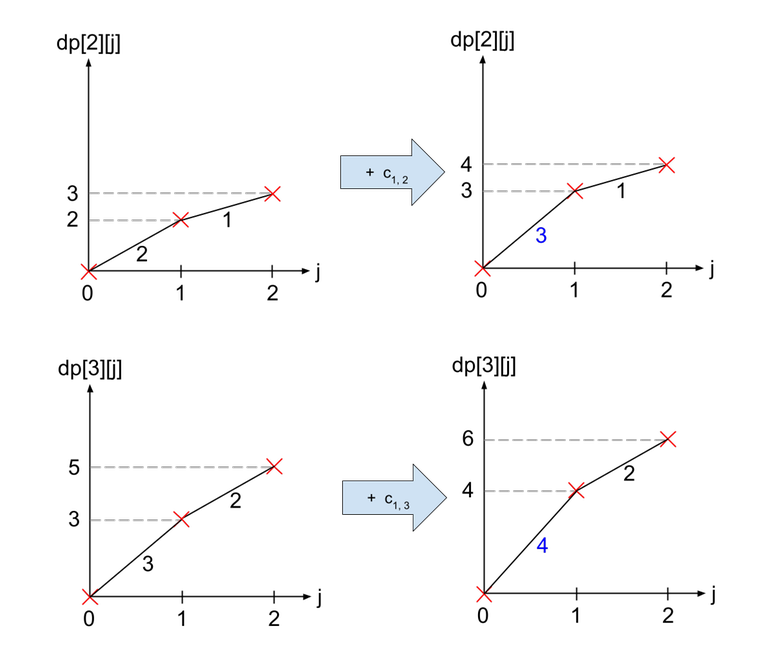
Let us see how we can obtain the graph of $$$dp[i]$$$ from $$$dp[i - 1]$$$. From the recurrence relation, we can see that $$$dp[i]$$$ is obtained by taking the minimum of the following 3 graphs: $$$dp[i - 1]$$$ shifted 1 to the right, $$$dp[i - 1]$$$ shifted $$$a_i$$$ upwards, and $$$dp[i - 1]$$$ shifted 1 to the left and $$$2a_i$$$ upwards.
As you can see in the image to the right, $$$dp[3]$$$ (shown in blue lines) can be formed by duplicating $$$dp[2]$$$ (shown in dotted lines) 3 times. Furthermore, the gradients of the resulting graph seems to be related to $$$a_i$$$.
Let us see how the dp function changes for a more complicated function. For this purpose, we will use the array $$$a = [1, 5, 5, 3, 6, 4]$$$. Supposed we have already calculated $$$dp[5]$$$ (shown in dotted lines) and want to calculate $$$dp[6]$$$.
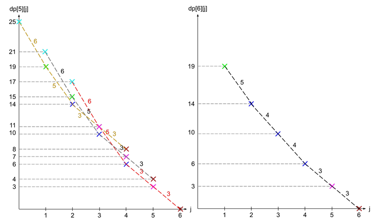
Note that the crosses are colour coded according to which $$$j$$$ it came from ($$$dp[5][1]$$$ is cyan, $$$dp[5][2]$$$ is green, $$$dp[5][3]$$$ is blue, $$$dp[5][4]$$$ is magenta, and $$$dp[5][5]$$$ is brown). We can see that as we compare the 3 overlapping graphs, the point where one graph starts to become the minimum is when the gradient becomes larger than $$$a_i$$$ (in this case $$$a_6 = 4$$$). Why is that so?
If we only compare the red and black line, we see that the difference between a point on the red line and the same coloured point on the black line (it is one spot to the left) always has a difference of $$$a_i$$$. This is because same coloured points comes from the same $$$dp[i - 1][j]$$$ and only differ from shifting upwards by $$$a_i$$$.
Hence, when we look from right to left, while the gradient of the red line is less than $$$a_i$$$, the red line is always optimal as the difference between two adjacent points on the red line is equal to the gradient while the difference between the adjacent points on the black line and red line is equal to $$$a_i$$$. The moment $$$a_i$$$ becomes smaller than the gradient, the black line becomes more optimal instead, and when we switch from the black line to red line, the new gradient in between the two lines is $$$a_i$$$ (see the blue points on the right graph).
Hence, if we store the gradients of $$$dp[i - 1]$$$ in a priority queue, all we need to do to transition to $$$dp[i]$$$ is to insert $$$a_i$$$ two times. However, since we do not want $$$dp[i][0]$$$, we can just pop out the largest gradient which represents $$$dp[i][0]$$$. Then after we are done processing $$$dp[n]$$$, the answer is just the sum of the gradients in the priority queue.
ARC123D — Inc, Dec — Decomposition
Abridged Statement
Given an array of $$$n$$$ numbers $$$a_1, a_2, \ldots, a_n$$$.
You want to construct two arrays $$$b_1, b_2, \ldots, b_n$$$ and $$$c_1, c_2, \ldots, c_n$$$ that satisfies the following conditions
- $$$a_i = b_i + c_i$$$ for all $$$1 \le i \le n$$$,
- $$$b$$$ is non-decreasing,
- $$$c$$$ is non-increasing
Find the minimum possible cost of $$$\sum_{i=1}^n(|b_i| + |c_i|)$$$
Ideas
We define $$$dp[i][j]$$$ as the minimum possible cost from $$$1$$$ to $$$i$$$ such that $$$b_i \le j$$$. By letting $$$b_i = k$$$ for each $$$k \le j$$$, we can come up with the following relation
$$$dp[i][j] = \max_{k \le j} (dp[i - 1][k - \max(0, a_i - a_{i - 1})] + |k| + |a_i - k|)$$$
The reason why we have $$$dp[i - 1][k - \max(0, a_i - a_{i - 1})]$$$ is to account for the non-increasing property of $$$c$$$. Let $$$k' = b_{i - 1}$$$ and $$$k = b_i$$$. Then, $$$c_{i - 1} = a_{i - 1} - k'$$$ and $$$c_i = a_i - k$$$. Since $$$c_{i -1} \ge c_i$$$, we have $$$a_{i - 1} - k' \ge a_i - k$$$, it simplifies to $$$k' \le k - (a_i - a_{i - 1})$$$.
Solution
Does the absolute signs remind you of 713C - Sonya and Problem Wihtout a Legend? If we plot the graph of $$$y = |x| + |a_i - x|$$$, we get

We observe that from $$$0$$$ to $$$a_i$$$, the line is horizontal at y coordinate of $$$a_i$$$ and on the left and right side of the horizontal line, the gradient is $$$-2$$$ and $$$2$$$ respectively. We can handle this easily by just inserting the slope-changing points into a priority queue.
Next, we have to handle $$$dp[i - 1][j - \max(0, a_i - a_{i - 1})]$$$. This means that we just have to offset the graph of $$$dp[i - 1]$$$ by $$$\max(0, a_i - a_{i - 1})$$$ units to the right. To do this, we just store an extra variable offsetwhich represents how much the original graph was shifted by.
Now, in order to combine both the shifted $$$dp[i - 1]$$$ and the $$$|j| + |a_i - j|$$$, we store all the slope changing points in a priority queue, offset the points, and then insert extra slope changing points at $$$0$$$ and $$$a_i$$$.
To illustrate this, we will use the array $$$a=[1, -2, 3]$$$. To move from $$$dp[2]$$$ to $$$dp[3]$$$, we first shift the graph of $$$dp[2]$$$ by $$$5$$$ units to the right. Then, we add on $$$y = |x| + |5 - x|$$$, which is shown below as the blue line.

For ease of implementation, observe that the slopes changes by 2 every time, so we can just let each point in the priority queue represent a change in 2 units of gradient.
RMI21 — Paths
Abridged Statement (Modified)
You have a tree of $$$n$$$ vertices. The weight of the $$$i$$$-th edge is equal to $$$c_i$$$. You want to select $$$k$$$ vertices such that the sum of the weights of all edges that lie on the path of vertex $$$1$$$ to any one of the $$$k$$$ vertices is maximised. Find the maximum possible sum.
- $$$1 \le k \le n \le 10^5$$$
- $$$0 \le c_i \le 10^9$$$
Ideas
It is obvious that we will only select the leaf nodes as they will cover all their parent nodes as well. We can come up with a $$$O(nk)$$$ dp solution easily. For each vertex $$$u$$$, let $$$dp[u][j]$$$ be the answer for the subtree of $$$u$$$ while selecting $$$j$$$ vertices.
For leaf vertices, we have $$$dp[u][0] = 0$$$. When we have multiple edges, we have a knapsack-like transition. For every edge $$$u \rightarrow v$$$ where $$$u$$$ is the parent of $$$v$$$ and the edge weight is $$$c$$$, $$$dp[u][j] = \max_{k \le j} dp[u][j - k] + dp[v][k] + (k > 0) \cdot c$$$. What this dp is doing is that if you choose at least one leaf in the subtree of $$$v$$$ (represented by boolean ($$$k > 0$$$)), then cost $$$c$$$ will be included in the final sum. Then, the remaining $$$j - k$$$ selected vertices can go to the other edges in the subtree of $$$u$$$.
As a side note, the whole dp works in ammortised $$$O(nk)$$$ due to distribution dp. If you do not know what it is you can go find some codeforces blog about it.
Solution
Of course, we will plot our dp function on a graph again. Suppose we have the following tree

Let us see how we can obtain $$$dp[1]$$$. First, we have to increase all $$$dp[v][j]$$$ by $$$c_{u, v}$$$ for all $$$j \ge 1$$$. We see that this operation is just increasing the first gradient by $$$c_{u, v}$$$.
To combine the two graphs, we realise that we are actually just combining the gradients of both graphs in decreasing order. In the diagram below, the blue lines represent the lines from $$$dp[2]$$$ and the orange lines represent the lines from $$$dp[3]$$$.
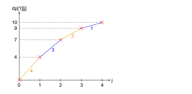
To implement this, we simply store a priority queue of the gradients at every vertex, then do small to large merging to calculate the new gradients for its parent.
Greedy Observation
Stare at the above code for a few seconds... Do you see the greedy that the code is effectively doing?
We are effectively assigning each edge $$$u \rightarrow v$$$ to the leaf which is the furthest distance from $$$v$$$, and then choosing the largest $$$k$$$ leaves at the end.
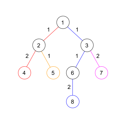
As we can see in the above diagram, edge $$$1 \rightarrow 3$$$ belongs to leaf $$$8$$$ as the distance from $$$3$$$ to $$$8$$$ is larger than the distance from $$$3$$$ to $$$7$$$. The same argument can be used for $$$1 \rightarrow 2$$$.
After assigning all the edges to the leaves, leaf $$$4$$$ has weight $$$3$$$, leaf $$$5$$$ has weight $$$1$$$, leaf $$$8$$$ has weight $$$4$$$, and leaf $$$7$$$ has weight $$$2$$$. So we simply select the $$$k$$$ largest weights and that will be our answer.
With this greedy observation, we can come up with an even simpler code which is faster as it does not require set merging. We can just keep a global set containing the weights of the leaves, and store an extra array $$$mx[u]$$$ containing the leaf with the maximum weight in the subtree of $$$u$$$.
You might be thinking, we already solved this problem, what's the point of the greedy observation?? Well... I tricked you and there is more to the problem.
Abridged Statement (Original)
You have a tree of $$$n$$$ vertices. The weight of the $$$i$$$-th edge is equal to $$$c_i$$$. For each root $$$\boldsymbol{r}$$$, you want to select $$$k$$$ vertices such that the sum of the weights of all edges that lie on the path of vertex $$$\boldsymbol{r}$$$ to any one of the $$$k$$$ vertices is maximised. Find the maximum possible sum for each root $$$\boldsymbol{r}$$$.
Solution
The final solution is a lot easier using the greedy observation. Since we want the answer for each root, we can simply do rerooting dp, maintaining 2 sets, one containing the largest $$$k$$$ elements and the other containing the remaining elements. We can easily update the sets, sums, and max while rerooting.
Since this is a slope trick blog, I will not cover the rerooting dp. You can read my code here to try to figure it out yourself if you are curious.
Bonus
Frisbee
(problem is from local judge so I will not attach the link to the question)
Abridged Statement
You are currently standing at point $$$(0, 0)$$$ of a grid. There are $$$n$$$ special points on the grid, each point being $$$(x_i, y_i)$$$. For each time $$$t$$$ from $$$1$$$ to $$$n$$$, you have to do one of the following:
- Move to any point with the same x-coordinate as point $$$t$$$. In other words, you have to move to a point $$$(x_t, a)$$$ where $$$a$$$ is any integer that you can choose.
- Move to any point with the same y-coordinate as point $$$t$$$. In other words, you have to move to a point $$$(a, y_t)$$$ where $$$a$$$ is any integer that you can choose.
Find the minimum possible manhattan distance that you travel after time $$$n$$$.
- $$$1 \le n \le 10^6$$$
- $$$-10^9 \le x_i, y_i \le 10^9$$$
Ideas
The first obvious observation is that there is no point moving in both x and y direction in 1 unit of time. In other words, if for time $$$i$$$ we decide to choose option 1 and we are currently at point $$$(a, b)$$$, we will move to point $$$(x_i, b)$$$ which will increase our total distance by $$$|x_i - a|$$$.
This will allow us to come up with a very simple dp. We have 2 dp functions $$$xdp[i][j]$$$ and $$$ydp[i][j]$$$ where $$$xdp[i][j]$$$ represents the minimum distance travelled to reach points from $$$1$$$ to $$$i$$$ and ending up at point $$$(x_i, j)$$$, while $$$ydp[i][j]$$$ represents the same thing but ending up at $$$(j, y_i)$$$. You can think of it as $$$xdp$$$ stores the answers for ending with operation 1 while $$$ydp$$$ stores the answer for operation 2.
Then, we can come up with the recurrence, $$$xdp[i][j] = \min(xdp[i - 1][j] + |x_{i - 1} - x_i|, ydp[i - 1][x_i] + |y_{i - 1} - j|)$$$ The first term is from simply doing operation 1 twice in a row, while the second term is from doing operation 2 in the $$$i - 1$$$ step and then doing operation 1. We can easily come up with something similar for $$$ydp$$$ but I will leave it as an exercise for the reader.
Solution
Since $$$j$$$ can go up to $$$10^9$$$, it obviously will not work. This is where the slope trick comes in. The first term is very easy to handle as it is just increasing $$$xdp$$$ by a constant. So if we have a graph of $$$xdp[i][j]$$$ against $$$j$$$, we are just shifting the graph upwards. The second function is also quite simple as it is just the absolute function ($$$y = |x - c|$$$) shifted upwards by another constant.
To store the graph, we simply store the set of points which forms the valleys (the red crosses in the diagram below). Then, in order to transition to the next states, we just have to do some lower_bound on the sets and erase some points from the sets.
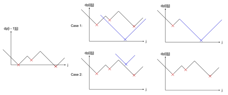
Make sure to only maintain the set of points which are the minimum. As you can see in case 2, the blue point that is added ended up to be useless as it is not the minimum, so we have to take care to not add it to the set. Furthermore, in case 1, we have to remove all the points that ends up being useless after the addition of the blue point. Take note that the removed points forms a continuous segment in the set.


