struct pt {
	int x, y;
	pt(int x_ = 0, int y_ = 0) : x(x_), y(y_) {}
	bool operator < (const pt p) const {
		if (x != p.x) return x < p.x;
		return y < p.y;
	}
	bool operator == (const pt p) const {
		return x == p.x and y == p.y;
	}
	pt operator + (const pt p) const { return pt(x+p.x, y+p.y); }
	pt operator - (const pt p) const { return pt(x-p.x, y-p.y); }
	pt operator * (const int c) const { return pt(x*c, y*c); }
	ll operator * (const pt p) const { return x*(ll)p.x + y*(ll)p.y; }
	ll operator ^ (const pt p) const { return x*(ll)p.y - y*(ll)p.x; }
	friend istream& operator >> (istream& in, pt& p) {
		return in >> p.x >> p.y;
	}
};

bool ccw(pt p, pt q, pt r) { // counter-clockwise
	return (q-p)^(r-q) > 0;
}

struct upper {
	set<pt> se;
	set<pt>::iterator it;

	int is_under(pt p) { // 1 -> inside ; 2 -> border
		it = se.lower_bound(p);
		if (it == se.end()) return 0;
		if (it == se.begin()) return p == *it ? 2 : 0;
		if (ccw(p, *it, *prev(it))) return 1;
		return ccw(p, *prev(it), *it) ? 0 : 2;
	}
	void insert(pt p) {
		if (is_under(p)) return;

		if (it != se.end()) while (next(it) != se.end() and !ccw(*next(it), *it, p))
			it = se.erase(it);
		if (it != se.begin()) while (--it != se.begin() and !ccw(p, *it, *prev(it)))
			it = se.erase(it);

		se.insert(p);
	}
};

struct dyn_hull { // 1 -> inside ; 2 -> border
	upper U, L;

	int is_inside(pt p) {
		int u = U.is_under(p), l = L.is_under({-p.x, -p.y});
		if (!u or !l) return 0;
		return max(u, l);
	}
	void insert(pt p) {
		U.insert(p);
		L.insert({-p.x, -p.y});
	}
	int size() {
		int ans = U.se.size() + L.se.size();
		return ans <= 2 ? ans/2 : ans-2;
	}
};

Hello, Codeforces!

I recently had to implement a dynamic convex hull (that supports insertions of points online), and I think the implementation got really small, comparable even to standard static convex hull implementations, and we get logarithmic inclusion query for free. We can:

1. Add a point to the convex hull in $$$\mathcal O(\log n)$$$ amortized time, with $$$n$$$ being the current hull size;
2. Check if some point belongs to the hull (or border) in $$$\mathcal O(\log n)$$$ time.

Upper Hull

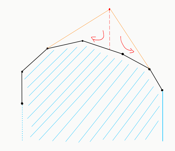
We can maintain the upper hull in a std::set (see below for image, upper hull is in black). We define the region that is under the upper hull as the region in blue, that is, the region that is, well... under. Note, however, that this region is open on the left.

To add a point (red) to the upper hull, we check if it is inside the blue region. If it is, we do nothing. If not, we need to add it, but we might need to remove some points so it continues to be convex. This is done by projecting the red point down (using lower_bound on our set) and iteratively removing points to the right and to the left, while they satisfy the corresponding direction condition.

struct pt {
	int x, y;
	pt(int x_ = 0, int y_ = 0) : x(x_), y(y_) {}
	bool operator < (const pt p) const {
		if (x != p.x) return x < p.x;
		return y < p.y;
	}
	bool operator == (const pt p) const {
		return x == p.x and y == p.y;
	}
	pt operator + (const pt p) const { return pt(x+p.x, y+p.y); }
	pt operator - (const pt p) const { return pt(x-p.x, y-p.y); }
	pt operator * (const int c) const { return pt(x*c, y*c); }
	ll operator * (const pt p) const { return x*(ll)p.x + y*(ll)p.y; }
	ll operator ^ (const pt p) const { return x*(ll)p.y - y*(ll)p.x; }
	friend istream& operator >> (istream& in, pt& p) {
		return in >> p.x >> p.y;
	}
};

bool ccw(pt p, pt q, pt r) { // counter-clockwise
	return (q-p)^(r-q) > 0;
}

struct upper {
	set<pt> se;
	set<pt>::iterator it;

	int is_under(pt p) { // 1 -> inside ; 2 -> border
		it = se.lower_bound(p);
		if (it == se.end()) return 0;
		if (it == se.begin()) return p == *it ? 2 : 0;
		if (ccw(p, *it, *prev(it))) return 1;
		return ccw(p, *prev(it), *it) ? 0 : 2;
	}
	void insert(pt p) {
		if (is_under(p)) return;

		if (it != se.end()) while (next(it) != se.end() and !ccw(*next(it), *it, p))
			it = se.erase(it);
		if (it != se.begin()) while (--it != se.begin() and !ccw(p, *it, *prev(it)))
			it = se.erase(it);

		se.insert(p);
	}
};

struct dyn_hull { // 1 -> inside ; 2 -> border
	upper U, L;

	int is_inside(pt p) {
		int u = U.is_under(p), l = L.is_under({-p.x, -p.y});
		if (!u or !l) return 0;
		return max(u, l);
	}
	void insert(pt p) {
		U.insert(p);
		L.insert({-p.x, -p.y});
	}
	int size() {
		int ans = U.se.size() + L.se.size();
		return ans <= 2 ? ans/2 : ans-2;
	}
};

bool ccw(pt p, pt q, pt r) { // counter-clockwise
	return (q-p)^(r-q) > 0;
}

struct upper {
	set<pt> se;
	set<pt>::iterator it;

	int is_under(pt p) { // 1 -> inside ; 2 -> border
		it = se.lower_bound(p);
		if (it == se.end()) return 0;
		if (it == se.begin()) return p == *it ? 2 : 0;
		if (ccw(p, *it, *prev(it))) return 1;
		return ccw(p, *prev(it), *it) ? 0 : 2;
	}
	void insert(pt p) {
		if (is_under(p)) return;

		if (it != se.end()) while (next(it) != se.end() and !ccw(*next(it), *it, p))
			it = se.erase(it);
		if (it != se.begin()) while (--it != se.begin() and !ccw(p, *it, *prev(it)))
			it = se.erase(it);

		se.insert(p);
	}
};

Convex Hull

Now, to implement the full convex hull, we just need an upper and lower hull. But we do not need to implement the lower hull from scratch: we can just rotate the points $$$\pi$$$ radians and store a second upper hull!

Be careful: if the hull has size 1, the point will be represented in both upper and lower hulls. If the hull has size at least 2, then both the first and last points in the upper hull will also appear in the lower hull (in last and first position, respectively). The size() function below is adjusted for this.

struct dyn_hull { // 1 -> inside ; 2 -> border
	upper U, L;

	int is_inside(pt p) {
		int u = U.is_under(p), l = L.is_under({-p.x, -p.y});
		if (!u or !l) return 0;
		return max(u, l);
	}
	void insert(pt p) {
		U.insert(p);
		L.insert({-p.x, -p.y});
	}
	int size() {
		int ans = U.se.size() + L.se.size();
		return ans <= 2 ? ans/2 : ans-2;
	}
};

Conclusion

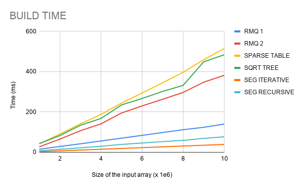
This implementation is considerably small and also not too slow (the constant factor of std::set operations is not small, but if is in function of the hull size, which in some applications can me small). We also get the logarithmic time query to check if some point is inside the hull.

Removing a point from the convex hull is much trickier, and since our runs in amortized logarithmic time, this can not be modified to support removals.

Hello, Codeforces!

I want to share with you 2 problems that I was not able to find a tight time complexity / bound for. After trying for a while, I decided to ask here, maybe someone can help me.

Problem 1

We want to maintain a collection of arrays of integers in $$$[0, U)$$$ represented with binary search trees, such as Treaps. We will have $$$q$$$ updates, which can be one of the following:

1. Split an array by position;
2. Concatenate two arrays;
3. Reverse an array;
4. Split an array by value.

Of course, it is well known how to support operations (1), (2) and (3) each in $$$\mathcal O(\log n)$$$, if $$$n$$$ is the total size of the collection.

What is interesting here is operation (4). Going into more detail about what it means, given an array and some value $$$x$$$, we want to split this array into two: one containing values that are smaller than $$$x$$$ in the same order as they were, and the other containing values that are at least $$$x$$$, also in the same order as they originally were. This is equivalent to running

std::stable_partition(v.begin(), v.end(), [&](int k) { return k < x; });

My proposed solution to implement this is to repeatedly split the array at the first position that has value smaller than $$$x$$$, then split at the first position that has value at least $$$x$$$, and repeat. It would look like this

void treap::partition(int x) {
	treap small, big;
	while (size()) {
		treap tmp;
		split(first_not_smaller(x), tmp);
		small.concat(tmp);
		split(first_smaller(x), tmp);
		big.concat(tmp);
	}
	// Now the elements are split into small and big,
	// and this treap is empty
}

The number of splits this algorithms does is the number of positions such that a "small" element and a "big" element are adjacent in the array.

Of course, this can be linear in the worst case, but can you find an instance such that this algorithm does $$$\Theta(q * n)$$$ splits? My guess is that this algoriths does at most $$$\mathcal O(\log U)$$$ splits, amortized. But I was not able to prove this.

I have tried a few potential functions, such as the sum of logs of gaps between adjacent values in the arrays, but they did not work.

Full code: link.

Problem 2

It turns out that a bound for this problem implies a bound for the previous problem, if we implement it in a specific way.

Imagine that there are $$$n$$$ coins, arranged in some piles in an arbitrary way. We will do $$$n$$$ operations. In each operation, we choose some number $$$k > 0$$$, and choose $$$k$$$ non-empty piles. For each of these piles, we choose a non-zero number of coins to take from it. All of the coins we took are arranged in a new pile.

The cost of the operation is $$$k$$$ (note that it is not the total number of coins, but the number of piles).

If we have the freedom to choose our operations in any way we like (and also the starting configuration), what is the maximum cost we can achieve? I could not find an instance that took $$$\Theta(n^2)$$$. However it is easy to create an instance that takes $$$\Theta(n * \sqrt n)$$$.

We think the maximum cost is $$$\mathcal O(n * \sqrt n)$$$, but we could not prove it. We managed, however, to prove this bound if we restrict the operation a bit: if we only allow to take at most one coin per pile.

Challenge

Can you prove any of the above unproven bounds? Can you find a counter-example? Please let me know, I will be happy to discuss this in the comments!

Hello, Codeforces!

Following the recent motivation of writing educational blogs thanks to peltorator (context), I decided to write another blog on strings, specifically on variations of the very classic String Matching Problem.

Prerequisites
1. KMP — cp-algorithms
2. Aho-Corasick — cp-algorithms
3. FFT — blog by -is-this-fft-

Throughout this blog, $$$n$$$ will be the size of the text (or sum of sizes of texts, if applicable), and $$$m$$$ will be the same for the pattern.

Simple Pattern Matching

Input: text $$$T$$$, pattern $$$P$$$.
Updates: none.
Query: in which positions does $$$P$$$ occur in $$$T$$$?

This is just KMP.

Complexity: $$$\mathcal O(n + m)$$$

Multiple Patterns

Input: text $$$T$$$, several patterns $$$P_i$$$.
Updates: none.
Query: what is the total number of occurrences of all $$$P_i$$$'s in $$$T$$$?

This is just Aho-Corasick.

Complexity: $$$\mathcal O((n + m) \log |\Sigma|)$$$

Adding and Removing Patterns

Input: several texts $$$T_i$$$, several patterns $$$P_j$$$.
Updates: add / remove pattern $$$P_j$$$ to a set $$$S$$$.
Query: what is the total number of occurrences of strings in $$$S$$$ in $$$T_i$$$?

This is 710F - String Set Queries.

Let's first consider only the addition of strings. What we can do is maintain several Aho-Corasick (AC) structures: for every $$$p$$$, we will have at most one AC with $$$2^p$$$ strings, so we have at most $$$\log m$$$ non-empty ACs. We will do this in the following manner: $$$p$$$'s with non-empty AC of size $$$2^p$$$ will be the binary representation of the number of strings we already added.

For example, if we currently have 6 strings, we will have one AC with 2 strings and another with 4 strings. So, how do we add a string? If we do not have an AC with size 1, we just create a new AC with this string. Now suppose there is already an AC with size one. If there is no AC with size 2, we just delete the AC with size 1 and create a new AC from scratch with these 2 strings. So it is basically binary incrementation: we take all strings in the suffix of active ACs, destroy the ACs and create a new AC with all these strings.

2 -> {v, w}
4 -> {r, s, t, u}

1 -> {x}
2 -> {v, w}
4 -> {r, s, t, u}

1 -> {y}
1 -> {x}
2 -> {v, w}
4 -> {r, s, t, u}

2 -> {x, y}
2 -> {v, w}
4 -> {r, s, t, u}

4 -> {v, w, x, y}
4 -> {r, s, t, u}

8 -> {r, s, t, u, v, w, x, y}

We can easily see that each string can be promoted at most $$$\log m$$$ times, and its contribution to the time complexity is its size times the number of times it is promoted. Therefore, we pay in total $$$\mathcal O(m \log m)$$$ time to build the ACs. For the query, we just sum over the query in all ACs, so this costs us $$$\mathcal O(n \log m)$$$ time.

Finally, to remove strings, just create another instance of this data structure and subtract the queries.

Complexity: $$$\mathcal O((n+m) \log m \log|\Sigma|)$$$
Code: 133199770

Pattern Query

Input: text $$$T$$$, several patterns $$$P_i$$$.
Updates: none.
Query: how many times does $$$P_i$$$ occur in $$$T$$$? This query needs to be answered online, that is, we do not know all $$$P_i$$$'s in advance.

This is the topic of this edu section.

This can be solved with suffix data structures. I will describe a solution using suffix array (SA). First we build the SA of the text. It is not hard to see that the indices of the matches of any pattern are contiguous in the SA, so we associate a pattern with this range (for the empty pattern, the range is $$$[0, n)$$$, and the range is empty for non-occurring patterns).

Now, to find the occurrences of $$$P_i$$$ in $$$T$$$, we process each character of $$$P_i$$$ at a time, and each time we possibly reduce our range. This is easy to do with binary search, since suffixes are sorted. At the end, the number of occurrences of $$$P_i$$$ in $$$T$$$ is the size of the range, and the actual occurrences are the values in the SA in this range.

Complexity: $$$\mathcal O(n + m \log n)$$$
Code: link

Dynamic Pattern

Input: text $$$T$$$, pattern $$$P$$$.
Updates: Change a character in $$$P$$$.
Query: how many times does $$$P$$$ occur in $$$T$$$?

This is a bit trickier and has a lot of nuances. It turns out that if we have the SA range associated with some pattern (and this pattern occurs in the text), we can update the pattern not only with character addition to the right, but also with character removal to the right, and character addition / removal to the left (we can remove several characters at once), all in $$$\mathcal O(\log n)$$$ via binary searches and LCP queries. In fact, if we have the ranges of two patterns, we can compute the range of the concatenation of these patterns in $$$\mathcal O(\log n)$$$!

This breaks if the pattern does not occur in the text, but we can fix this by representing "maximal" occurring pattern substrings: a partition of the pattern such that every part occurs in the text (or is a single character that does not occur), but the concatenation of adjacent parts does not occur. We can maintain this partition in a Treap, for example, and this property is easy to maintain.

To answer the query, if the size of the partition is greater than one, the answer is zero, otherwise it is the size of the single range.

I might write a blog describing how to do this in detail in the future.

Complexity: $$$\mathcal O((n+m) \log (n + m))$$$
Code: 136951123

Dynamic Text

Input: text $$$T$$$, several patterns $$$P_i$$$.
Updates: Add / remove a character to the beginning of $$$T$$$.
Query: how many times does $$$P_i$$$ occur in $$$T$$$?

It turns out that we can maintain the SA of the text under these updates. I explained how to do this in [Tutorial] Dynamic Suffix Arrays.

Complexity: $$$\mathcal O((n+m) \log n)$$$

At most $$$k$$$ mismatches

Input: text $$$T$$$, pattern $$$P$$$, integer $$$k$$$.
Updates: none.
Query: how many times does $$$P$$$ occur in $$$T$$$, allowing for at most $$$k$$$ character mismatches in each match?

We will solve this using polynomials. Let's compute, for every character in our alphabet $$$\Sigma$$$, the number of characters that the pattern matches with the text for every possible starting position of a match. For example, if the pattern is $$$\tt aba$$$ and the text is $$$\tt aaba$$$, we would like to know that the character $$$\tt a$$$ has one match at position 0 and two at position 1, and for $$$\tt b$$$, zero at position 0 and one at position 1.

So let's fix some character $$$c$$$. We define a polynomial $$$R_c(x) = \sum_i [T[i] == c] x^i$$$, that is, we consider only the positions that are equal to $$$c$$$ in the text. We do the same for the pattern, but reversed: $$$S_c(x) = \sum_i [P[i] == c] x^{|P|-1-i}$$$. It is not hard to see that the coefficient of $$$x^{|P|-1}$$$ of $$$R*S$$$ is equal to the number of characters $$$c$$$ that match if we try to match $$$P$$$ at position 0 in $$$T$$$, the coefficient of $$$x^{|P|}$$$ of $$$R*S$$$ is equal to the number of characters $$$c$$$ that match if we try to match $$$P$$$ at position 1 in $$$T$$$, and so on.

Now we just do this for every character and add the result, and we have how many characters match at every position. This requires $$$|\Sigma|$$$ polynomial multiplications, so we can achieve $$$\mathcal O(|\Sigma| (n+m) \log (n + m))$$$ using FFT.

Complexity: $$$\mathcal O(|\Sigma| (n+m) \log (n + m))$$$

Wildcards

Input: text $$$T$$$, pattern $$$P$$$. Pattern and text may have wildcards, that match with any other character.
Updates: none.
Query: in which positions does $$$P$$$ occur in $$$T$$$?

This solution is described in https://www.informatika.bg/resources/StringMatchingWithFFT.pdf, and it also uses polynomials. First, if we did not have wildcards, one way to solve matching with FFT is to compute, for every $$$i$$$:

If this value is zero, then all the terms are zero, so we have a match a position $$$i$$$. Now we can expand this out:

The first term does not depend on $$$i$$$, so we can trivially precompute it. The last term is also easy to compute, via prefix sums. The middle term can be computed using polynomial multiplication (FFT), as we did on the last problem.

Not we introduce wildcards. If we define the value of the characters such that the wildcard is zero and the other character are positive, we can see that, for matching at position $$$i$$$,

Gives us what we want: for this to be zero, every term has to be zero, so every character either matches or at least one is a wildcard, which is exactly what we wanted. Expanding it, we get:

Each of these 3 terms can be computed using FFT: if $$$R$$$ and $$$S$$$ are the polynomials associated with $$$P$$$ and $$$T$$$, respectively (like in the previous problem) the first term can be computed as $$$\lbrace r_i^3\rbrace * S$$$, the second as $$$\lbrace r_i^2\rbrace * \lbrace s_i^2\rbrace $$$, and the last as $$$R * \lbrace s_i^3\rbrace $$$. Here $$$\lbrace r_i^3\rbrace$$$ means cubing each term of the polynomial. We sum this up for each term that we want to check and if we get zero, this means we have a match.

Complexity: $$$\mathcal O((n+m) \log (n + m))$$$
Code: link

Conclusion

We have seen several variations of the String Matching Problem. Other variations can get very complicated very quickly, such as trying to update an arbitrary position in the text and maintain, for example, its Suffix Array.

I hope you could learn something from this blog, and feel free to ask for more details on specific parts if needed.

Hello, Codeforces!

In this blog I will describe yet another useless unconventional data structure. This time, I will show how to maintain an extended suffix array (suffix array, inverse of suffix array, and $$$lcp$$$ array) while being able to add or remove some character at the beginning of the string in $$$\mathcal{O}(\log n)$$$ amortized time.

It can be used to overkill solve problem M from 2020-2021 ACM-ICPC Latin American Regionals, which my team couldn't solve during the contest. I learned it from here (Chinese), but it is not shown how to maintain the $$$lcp$$$ array.

Here is the whole code of the data structure. To read this blog, I recommend you ignore this code for now, but use it if you have questions about helper functions, constructors, etc, since I will pass over some implementation details in the explanations.

struct dyn_sa {
	struct node {
		int sa, lcp;
		node *l, *r, *p;
		int sz, mi;
		node(int sa_, int lcp_, node* p_) : sa(sa_), lcp(lcp_),
			l(NULL), r(NULL), p(p_), sz(1), mi(lcp) {}
		void update() {
			sz = 1, mi = lcp;
			if (l) sz += l->sz, mi = min(mi, l->mi);
			if (r) sz += r->sz, mi = min(mi, r->mi);
		}
	};

	node* root;
	vector<ll> tag; // tag of a suffix (reversed id)
	string s; // reversed

	dyn_sa() : root(NULL) {}
	dyn_sa(string s_) : dyn_sa() {
		reverse(s_.begin(), s_.end());
		for (char c : s_) push_front(c);
	}
	~dyn_sa() {
		vector<node*> q = {root};
		while (q.size()) {
			node* x = q.back(); q.pop_back();
			if (!x) continue;
			q.push_back(x->l), q.push_back(x->r);
			delete x;
		}
	}

	int size(node* x) { return x ? x->sz : 0; }
	int mirror(int i) { return s.size()-1 - i; }
	bool cmp(int i, int j) {
		if (s[i] != s[j]) return s[i] < s[j];
		if (i == 0 or j == 0) return i < j;
		return tag[i-1] < tag[j-1];
	}
	void fix_path(node* x) { while (x) x->update(), x = x->p; }
	void flatten(vector<node*>& v, node* x) {
		if (!x) return;
		flatten(v, x->l);
		v.push_back(x);
		flatten(v, x->r);
	}
	void build(vector<node*>& v, node*& x, node* p, int L, int R, ll l, ll r) {
		if (L > R) return void(x = NULL);
		int M = (L+R)/2;
		ll m = (l+r)/2;
		x = v[M];
		x->p = p;
		tag[x->sa] = m;
		build(v, x->l, x, L, M-1, l, m-1), build(v, x->r, x, M+1, R, m+1, r);
		x->update();
	}
	void fix(node*& x, node* p, ll l, ll r) {
		if (3*max(size(x->l), size(x->r)) <= 2*size(x)) return x->update();
		vector<node*> v;
		flatten(v, x);
		build(v, x, p, 0, v.size()-1, l, r);
	}
	node* next(node* x) {
		if (x->r) {
			x = x->r;
			while (x->l) x = x->l;
			return x;
		}
		while (x->p and x->p->r == x) x = x->p;
		return x->p;
	}
	node* prev(node* x) {
		if (x->l) {
			x = x->l;
			while (x->r) x = x->r;
			return x;
		}
		while (x->p and x->p->l == x) x = x->p;
		return x->p;
	}

	int get_lcp(node* x, node* y) {
		if (!x or !y) return 0; // change defaut value here
		if (s[x->sa] != s[y->sa]) return 0;
		if (x->sa == 0 or y->sa == 0) return 1;
		return 1 + query(mirror(x->sa-1), mirror(y->sa-1));
	}
	void add_suf(node*& x, node* p, int id, ll l, ll r) {
		if (!x) {
			x = new node(id, 0, p);
			node *prv = prev(x), *nxt = next(x);
			int lcp_cur = get_lcp(prv, x), lcp_nxt = get_lcp(x, nxt);
			if (nxt) nxt->lcp = lcp_nxt, fix_path(nxt);
			x->lcp = lcp_cur;
			tag[id] = (l+r)/2;
			x->update();
			return;
		}
		if (cmp(id, x->sa)) add_suf(x->l, x, id, l, tag[x->sa]-1);
		else add_suf(x->r, x, id, tag[x->sa]+1, r);
		fix(x, p, l, r);
	}
	void push_front(char c) {
		s += c;
		tag.push_back(-1);
		add_suf(root, NULL, s.size() - 1, 0, 1e18);
	}

	void rem_suf(node*& x, int id) {
		if (x->sa != id) {
			if (tag[id] < tag[x->sa]) return rem_suf(x->l, id);
			return rem_suf(x->r, id);
		}
		node* nxt = next(x);
		if (nxt) nxt->lcp = min(nxt->lcp, x->lcp), fix_path(nxt);

		node *p = x->p, *tmp = x;
		if (!x->l or !x->r) {
			x = x->l ? x->l : x->r;
			if (x) x->p = p;
		} else {
			for (tmp = x->l, p = x; tmp->r; tmp = tmp->r) p = tmp;
			x->sa = tmp->sa, x->lcp = tmp->lcp;
			if (tmp->l) tmp->l->p = p;
			if (p->l == tmp) p->l = tmp->l;
			else p->r = tmp->l;
		}
		fix_path(p);
		delete tmp;
	}
	void pop_front() {
		if (!s.size()) return;
		s.pop_back();
		rem_suf(root, s.size());
		tag.pop_back();
	}
	
	int query(node* x, ll l, ll r, ll a, ll b) {
		if (!x or tag[x->sa] == -1 or r < a or b < l) return s.size();
		if (a <= l and r <= b) return x->mi;
		int ans = s.size();
		if (a <= tag[x->sa] and tag[x->sa] <= b) ans = min(ans, x->lcp);
		ans = min(ans, query(x->l, l, tag[x->sa]-1, a, b));
		ans = min(ans, query(x->r, tag[x->sa]+1, r, a, b));
		return ans;
	}
	int query(int i, int j) { // lcp(s[i..], s[j..])
		if (i == j) return s.size() - i;
		ll a = tag[mirror(i)], b = tag[mirror(j)];
		int ret = query(root, 0, 1e18, min(a, b)+1, max(a, b));
		return ret;
	}
	// optional: get isa[i], sa[i] and lcp[i] (standard index representation)
	int isa(int i) {
		i = mirror(i);
		node* x = root;
		int ret = 0;
		while (x) {
			if (tag[x->sa] < tag[i]) {
				ret += size(x->l)+1;
				x = x->r;
			} else x = x->l;
		}
		return ret;
	}
	// returns a pair with SA[i] and lcp[i]
	pair<int, int> operator[](int i) {
		node* x = root;
		while (1) {
			if (i < size(x->l)) x = x->l;
			else {
				i -= size(x->l);
				if (!i) return {mirror(x->sa), x->lcp};
				i--, x = x->r;
			}
		}
	}
};

1. Definitions

I will assume the reader is familiar with the definition of suffix array ($$$SA$$$) and $$$lcp$$$ array. If that is not the case, I recommend learning it from Codeforces EDU.

Here, the $$$i$$$-th position of the $$$lcp$$$ array will denote the longest common prefix between $$$SA[i]$$$ and $$$SA[i-1]$$$. Also, $$$lcp[0] = 0$$$. The inverse suffix array ($$$ISA$$$), or rank of a suffix says what position that suffix is at in the $$$SA$$$. That is, $$$ISA[SA[i]] = i$$$.

In the data structure, since we add characters at the front of the string, we will use a reversed index representation of each suffix. For example, the suffix of index 2 of $$$baabac$$$ is $$$bac$$$. We will use a function $$$\texttt{mirror}$$$ to go from the standard index representation to the reversed one, and vice versa.

int mirror(int i) {
	return s.size()-1 - i;
}

2. Binary search tree

Let's represent the $$$SA$$$ using a binary search tree, such that the in-order traversal of the tree gives the $$$SA$$$. For example, take the $$$SA$$$ of $$$baabac$$$ below. For each suffix, its (reversed) index and $$$lcp$$$ are represented.

We could represent this using the following binary search tree.

Additionally, we will store an array $$$tag$$$, such that $$$tag[i] < tag[j]$$$ if, and only if, suffix $$$i$$$ comes before suffix $$$j$$$ in the $$$SA$$$ (equivalently, in the binary search tree). Using this, we can compare two suffixes lexicographically in constant time. This is pivotal to make the complexity of the operations $$$\mathcal{O}(\log n)$$$ amortized.

Because we want to maintain the $$$tag$$$ array, we will not use a binary search tree that does rotations, since it not trivial how to update the $$$tag$$$ values during the rebalancing. Instead, we will use a binary search tree called Amortized weight-balanced trees (see below for references). The idea of these trees is that, at any point, every subtree will be $$$\alpha$$$-balanced for some $$$0.5 < \alpha < 1$$$, which means that for every subtree rooted at node $$$x$$$, $$$\max(\text{size}(x.left), \text{size}(x.right)) \leq \alpha \cdot \text{size}(x)$$$. It turns out that if we insert and delete using trivial binary search tree algorithms and, after every change, for every node that is not $$$\alpha$$$-balanced we simply rebuild the entire subtree rooted at that node so that it becomes as balanced as possible, the height of the tree and the amortized cost of inserting and deleting is $$$\mathcal{O}(\log_{\frac{1}{\alpha}} n)$$$. Proving this is beyond the scope of this blog. In the code, I use $$$\alpha = 2/3$$$.

This rebuilding scheme makes it easy to maintain the $$$tag$$$ values by having a large enough interval of possible values (I use $$$[0, 10^{18}]$$$) and recursively dividing it in half (refer to the code for more details).

Given that we have a binary search tree representing the $$$SA$$$ and $$$lcp$$$ array with logarithmic height, how do we query for $$$SA$$$, $$$lcp$$$ and $$$ISA$$$? If we maintain the subtree sizes of the tree, we simply go down the tree to get the $$$i$$$-th smallest node and so we get $$$SA[i]$$$ and $$$lcp[i]$$$ in $$$\mathcal{O}(\log n)$$$, if $$$n$$$ is the size of the string. To get $$$ISA[i]$$$, we go down the tree, counting how many nodes in the tree have $$$tag$$$ value smaller than $$$tag[i]$$$.

// functions to be called with standard index representation
int isa(int i) {
	i = mirror(i);
	node* x = root;
	int ret = 0;
	while (x) {
		if (tag[x->sa] < tag[i]) {
			ret += size(x->l)+1;
			x = x->r;
		} else x = x->l;
	}
	return ret;
}
// returns a pair with SA[i] and lcp[i]
pair<int, int> operator[](int i) {
	node* x = root;
	while (1) {
		if (i < size(x->l)) x = x->l;
		else {
			i -= size(x->l);
			if (!i) return {mirror(x->sa), x->lcp};
			i--, x = x->r;
		}
	}
}

Finally, we can also use the tree to query for the $$$lcp$$$ between two arbitrary suffixes $$$i$$$ and $$$j$$$ (not necessarily consecutive in the $$$SA$$$). We know that this is equal to the minimum between the $$$lcp$$$ values in the range defined by the two suffixes. So we just need to store the minimum over all $$$lcp$$$ values on every subtree, and query for the minimum over all nodes that have $$$tag$$$ value in the range $$$(tag[i], tag[j]]$$$, assuming $$$tag[i] < tag[j]$$$. This can be done by going down the tree similar to a segment tree, in $$$\mathcal{O}(\log n)$$$ time.

int query(node* x, ll l, ll r, ll a, ll b) {
	// current subtree can have tag values in the range [l, r]
	if (!x or tag[x->sa] == -1 or r < a or b < l) return s.size();
	if (a <= l and r <= b) return x->mi;
	int ans = s.size();
	if (a <= tag[x->sa] and tag[x->sa] <= b) ans = min(ans, x->lcp);
	ans = min(ans, query(x->l, l, tag[x->sa]-1, a, b));
	ans = min(ans, query(x->r, tag[x->sa]+1, r, a, b));
	return ans;
}
int query(int i, int j) { // lcp(s[i..], s[j..]) in standard index representation
	if (i == j) return s.size() - i;
	ll a = tag[mirror(i)], b = tag[mirror(j)];
	int ret = query(root, 0, 1e18, min(a, b)+1, max(a, b));
	return ret;
}

3. Adding a character

Since we add or remove characters at the front of the string, we only add or remove a single suffix of the string (and, equivalently, a single node in the binary search tree), and the previous suffixes remain unchanged and maintain their relative order. Below we see represented in red what changes in the $$$SA$$$ and $$$lcp$$$ after adding $$$b$$$ to $$$aabac$$$.

$$$\hspace{30pt}$$$

So, to update the structure with the new suffix, we just need to find the position where the new suffix will end up at, its $$$lcp$$$ value and we might need to update the $$$lcp$$$ value of the suffix that comes just after the added suffix.

3.1. Comparing the new suffix with another suffix

If we can compare the new suffix with any other suffix, we can use this to go down the tree and figure out the position we need to insert the new suffix. To make this comparison, we use the following trick: we compare the first character of the suffixes. If they are different, we know which one is smaller lexicographically. If they are the same, then we end up with a comparison between two suffixes that are already in the tree, and we know how to compare them! Just use their $$$tag$$$ value.

bool cmp(int i, int j) {
	if (s[i] != s[j]) return s[i] < s[j];
	if (i == 0 or j == 0) return i < j;
	return tag[i-1] < tag[j-1];
}

3.2. Getting the $$$lcp$$$ values

To get the $$$lcp$$$ value for the new suffix and for the node the goes after the new suffix (since its $$$lcp$$$ value might change), we will use the same trick: if the first characters of the suffixes are different, then their $$$lcp$$$ is zero. Otherwise, we are left with an $$$lcp$$$ query between two suffixes that are already in the quill, which we already know how to answer, just call the $$$\texttt{query}$$$ function.

int get_lcp(node* x, node* y) { // node x comes before node y in the tree
	if (!x or !y) return 0; // 0 by default
	if (s[x->sa] != s[y->sa]) return 0;
	if (x->sa == 0 or y->sa == 0) return 1;
	return 1 + query(mirror(x->sa-1), mirror(y->sa-1));
}

Since now we know how to compare the new suffix with any other suffix in the tree, and how to get the $$$lcp$$$ between the new suffix and any other suffix in the tree, we are ready to insert a new suffix: just go down the tree to the correct position, insert the new suffix, compute its $$$lcp$$$ and recompute the $$$lcp$$$ of the next node in the tree.

// [l, r] is the tag range of the current subtree
void add_suf(node*& x, node* p, int id, ll l, ll r) {
	if (!x) {
		x = new node(id, 0, p);
		// previous node and next node in the tree
		node *prv = prev(x), *nxt = next(x); 
		int lcp_cur = get_lcp(prv, x), lcp_nxt = get_lcp(x, nxt);
		// fix_path goes up to the rood calling update on the nodes
		if (nxt) nxt->lcp = lcp_nxt, fix_path(nxt);
		x->lcp = lcp_cur;
		tag[id] = (l+r)/2;
		x->update();
		return;
	}
	if (cmp(id, x->sa)) add_suf(x->l, x, id, l, tag[x->sa]-1);
	else add_suf(x->r, x, id, tag[x->sa]+1, r);
	fix(x, p, l, r); // update and rebuild subtree if unbalanced
}
void push_front(char c) {
	s += c;
	tag.push_back(-1);
	add_suf(root, NULL, s.size() - 1, 0, 1e18);
}

4. Removing a character

Removing a suffix is relatively straightforward: go down the tree, using the $$$tag$$$ array, to find where the suffix we want to remove is. When found, just remove it using standard binary search tree algorithm.

Now note that the $$$lcp$$$ value of the node that comes after the removed node might be incorrect. Luckily, it is easy to get its correct value: it is the minimum between the current value and the $$$lcp$$$ value of the suffix we are removing. This follows from the fact that the $$$lcp$$$ between two suffixes is the minimum over the $$$lcp$$$ values of the range defined by them in the $$$SA$$$.

void rem_suf(node*& x, int id) {
	if (x->sa != id) {
		if (tag[id] < tag[x->sa]) return rem_suf(x->l, id);
		return rem_suf(x->r, id);
	}
	node* nxt = next(x);
	// update the lcp value for the next node
	if (nxt) nxt->lcp = min(nxt->lcp, x->lcp), fix_path(nxt);
	node *p = x->p, *tmp = x;
	if (!x->l or !x->r) { // remove x directly
		x = x->l ? x->l : x->r;
		if (x) x->p = p;
	} else { // replace x by the node that comes before it
		for (tmp = x->l, p = x; tmp->r; tmp = tmp->r) p = tmp;
		x->sa = tmp->sa, x->lcp = tmp->lcp;
		if (tmp->l) tmp->l->p = p;
		if (p->l == tmp) p->l = tmp->l;
		else p->r = tmp->l;
	}
	fix_path(p);
	delete tmp;
}
void pop_front() {
	if (!s.size()) return;
	s.pop_back();
	rem_suf(root, s.size());
	tag.pop_back();
}

Note that I don't do the rebalancing/rebuilding stuff on the node deletion. This makes so the height of the tree won't always be logarithmic on the current size of the string, however it will still be logarithmic on the maximum size of the string so far, so this is not a problem.

5. Problems

I only know of one problem that makes sense using this data structure to solve it.

• 103185M - May I Add a Letter?

6. Final remarks

This data structure is relatively simple, and yet very powerful. Not even suffix trees and suffix automaton, that can update their structure with character additions, are capable of rollbacks without breaking their complexity. So this scores yet another point for suffix arrays being the best suffix structure.

This data structure is not too fast, but it is not super slow either. It runs in about 3 times the time of my static $$$\mathcal{O}(n \log n)$$$ suffix array implementation.

I would like to thank arthur.nascimento for creating the problem 103185M - May I Add a Letter?, which made me look into this data structure. Also tdas for showing me the existence of it.

References

Explanation of the data structure (without maintaining the $$$lcp$$$ array) (Chinese): Link

On the binary search tree used: Link1 Link2

Hello, Codeforces!

This blog is heavily inspired by TLE's blog using merging segment tree to solve problems about sorted list. I don't know exactly how well known this data structure is, but I thought it would be nice to share it anyway, along with some more operations that are possible with it.

What it can do

We want a data structure that we can think of a set/multiset of non-negative integers, or even as a sorted array. We want to support all of the following operations:

1. Create an empty structure;
2. Insert an element to the structure;
3. Remove an element from the structure;
4. Print the $$$k$$$'th smallest element (if we think of the structure as a sorted array $$$a$$$, we are asking for $$$a[k]$$$);
5. Print how many numbers less than $$$x$$$ there are in the set (similar to lower_bound in a std::vector);
6. Split the structure into two: one containing the $$$k$$$ smallest elements, and the other containing the rest;
7. Merge two structures into one (no extra conditions required).

Turns out that, if all elements are not greater than $$$N$$$, we can perform any sequence of $$$t$$$ such operations in $$$\mathcal{O}(t \log N)$$$, meaning that each operation costs $$$\mathcal{O}(\log N)$$$ amortized (as we will see, all operations except for (7) have worst case $$$\mathcal{O}(\log N)$$$).

How it works

We are going to use a dynamic segment tree to represent the elements. Think of each of them as an index, a leaf on a segment tree. We want the segment tree do be dynamic (we only create the nodes when we need them).

So, initially, there are no nodes on the structure (grey nodes are not present in the structure):

If we insert the value $$$2$$$, we need to create the path from the root to the leaf that represents $$$2$$$. It is also useful to store, on each node, the number of created leafs on that node's subtree.

Let's also add $$$1$$$, $$$4$$$ and $$$5$$$. In the end, the tree will look like this:

Using this representation, it is very straightforward to implement operations (1), (2) and (3). Operations (4) and (5) are also easy, they are classic segtree operations. To do operation (6), we can go down the tree and either call recursively to the left or right child. Here is a pseudocode of this operation:

node* split(node*& i, int k) {
    if (!k or !i) return NULL;
    node* ret = new node();
    if (i is a leaf) {
        i->cnt -= k; // assuming multiset
        ret->cnt += k;
    } else {
        if (k <= i->left->cnt) ret->left = split(i->left, k); // split the left
        else { // take everything from the left and split the right
            ret->left = i->left;
            ret->right = split(i->right, k - i->left->cnt);
            i->left = NULL;
        }
    }
    return ret;
}

It is clear that all these operations cost $$$\mathcal{O}(\log N)$$$. On operation (6), note that we only go down recursively to the left or to the right child.

But what about operation (7)? It turns out that we can merge two structures in the following way: to merge the subtrees defined by nodes l and r, if one of them is empty, just return the other. Otherwise, recursively merge l->left and r->left, and l->right and r->right. After that, we can delete either l or r, because they are now redundant: we only need one of them.

Now let's see why any sequence of $$$t$$$ operations will take $$$\mathcal{O}(t \log N)$$$ time. The number of nodes we create is bounded by $$$\mathcal{O}(t \log N)$$$, because each operation creates at most $$$\mathcal{O}(\log N)$$$ nodes. Now note that the merge algorithm either returns in $$$\mathcal{O}(1)$$$, or it deletes one node. So total number of times the algorithm doesn't return in $$$\mathcal{O}(1)$$$ is bounded by the total number of created nodes, so it is $$$\mathcal{O}(t \log N)$$$.

Implementation

There are some implementation tricks that make the code easier to write and use. Firstly, we don't need to set $$$N$$$ as a constant. Instead, we can have $$$N = 2^k-1$$$ for some $$$k$$$, and if we want to insert an element larger than $$$N$$$, we can just increase $$$k$$$, and update the segment tree (we will only need to create a new root, and set its left child to the old root).

Also, it's easy to change between set and multiset representation. It is also easy to insert $$$x$$$ occurrences of an element at once, just increase the cnt variable of the respective leaf accordingly.

This implementation uses $$$\mathcal{O}(t \log N)$$$ of memory, for $$$t$$$ operations.

template<typename T, bool MULTI=false, typename SIZE_T=int> struct sms {
	struct node {
		node *l, *r; // left and right childs
		SIZE_T cnt; // subtree leaf count
		node() : l(NULL), r(NULL), cnt(0) {}
		void update() { // update subtree leaf count
			cnt = 0;
			if (l) cnt += l->cnt;
			if (r) cnt += r->cnt;
		}
	};

	node* root;
	T N;

	sms() : root(NULL), N(0) {}
	sms(T v) : sms() { while (v >= N) N = 2*N+1; }
	sms(const sms& t) : root(NULL), N(t.N) { // copy - O(t log(N))
		for (SIZE_T i = 0; i < t.size(); i++) {
			T at = t[i];
			SIZE_T qt = t.count(at);
			insert(at, qt);
			i += qt-1;
		}
	}
	sms(initializer_list<T> v) : sms() { for (T i : v) insert(i); }
	~sms() {
		vector<node*> q = {root};
		while (q.size()) {
			node* x = q.back(); q.pop_back();
			if (!x) continue;
			q.push_back(x->l), q.push_back(x->r);
			delete x;
		}
	}

	friend void swap(sms& a, sms& b) { // O(1) swap
		swap(a.root, b.root), swap(a.N, b.N);
	}
	SIZE_T size() const { return root ? root->cnt : 0; }
	SIZE_T count(node* x) const { return x ? x->cnt : 0; }
	void clear() {
		sms tmp;
		swap(*this, tmp);
	}
	void expand(T v) { // increase N so value 'v' will fit
		for (; N < v; N = 2*N+1) if (root) {
			node* nroot = new node();
			nroot->l = root;
			root = nroot;
			root->update();
		}
	}

	node* insert(node* at, T idx, SIZE_T qt, T l, T r) {
		if (!at) at = new node();
		if (l == r) {
			at->cnt += qt;
			if (!MULTI) at->cnt = 1;
			return at;
		}
		T m = l + (r-l)/2;
		if (idx <= m) at->l = insert(at->l, idx, qt, l, m);
		else at->r = insert(at->r, idx, qt, m+1, r);
		return at->update(), at;
	}
	void insert(T v, SIZE_T qt=1) { // insert 'qt' occurrences of 'v'
		if (qt <= 0) return erase(v, -qt);
		assert(v >= 0);
		expand(v);
		root = insert(root, v, qt, 0, N);
	}

	node* erase(node* at, T idx, SIZE_T qt, T l, T r) {
		if (!at) return at;
		if (l == r) at->cnt = at->cnt < qt ? 0 : at->cnt - qt;
		else {
			T m = l + (r-l)/2;
			if (idx <= m) at->l = erase(at->l, idx, qt, l, m);
			else at->r = erase(at->r, idx, qt, m+1, r);
			at->update();
		}
		if (!at->cnt) delete at, at = NULL; // 'cnt' is always positive
		return at;
	}
	void erase(T v, SIZE_T qt=1) { // erase 'qt' occurrences of 'v'
		if (v < 0 or v > N or !qt) return;
		if (qt < 0) insert(v, -qt);
		root = erase(root, v, qt, 0, N);
	}
	void erase_all(T v) { // remove all occurrences of 'v'
		if (v < 0 or v > N) return;
		root = erase(root, v, numeric_limits<SIZE_T>::max(), 0, N);
	}

	SIZE_T count(node* at, T a, T b, T l, T r) const {
		if (!at or b < l or r < a) return 0;
		if (a <= l and r <= b) return at->cnt;
		T m = l + (r-l)/2;
		return count(at->l, a, b, l, m) + count(at->r, a, b, m+1, r);
	}
	SIZE_T count(T v) const { return count(root, v, v, 0, N); }
	SIZE_T order_of_key(T v) { return count(root, 0, v-1, 0, N); }
	SIZE_T lower_bound(T v) { return order_of_key(v); }

	const T operator [](SIZE_T i) const { // i-th smallest element (0 -> smallest)
		assert(i >= 0 and i < size());
		node* at = root;
		T l = 0, r = N;
		while (l < r) {
			T m = l + (r-l)/2;
			if (count(at->l) > i) at = at->l, r = m;
			else {
				i -= count(at->l);
				at = at->r; l = m+1;
			}
		}
		return l;
	}

	node* merge(node* l, node* r) {
		if (!l or !r) return l ? l : r;
		if (!l->l and !l->r) { // 'l' is a leaf
			if (MULTI) l->cnt += r->cnt;
			delete r;
			return l;
		}
		l->l = merge(l->l, r->l), l->r = merge(l->r, r->r);
		l->update(), delete r;
		return l;
	}
	void merge(sms& s) { // merge two sets
		if (N > s.N) swap(*this, s);
		expand(s.N);
		root = merge(root, s.root);
		s.root = NULL;
	}

	node* split(node*& x, SIZE_T k) {
		if (k <= 0 or !x) return NULL;
		node* ret = new node();
		if (!x->l and !x->r) x->cnt -= k, ret->cnt += k;
		else {
			if (k <= count(x->l)) ret->l = split(x->l, k);
			else {
				ret->r = split(x->r, k - count(x->l));
				swap(x->l, ret->l);
			}
			ret->update(), x->update();
		}
		if (!x->cnt) delete x, x = NULL; // 'cnt' is always positive
		return ret;
	}
	void split(SIZE_T k, sms& s) { // get the 'k' smallest elements
		s.clear();
		s.root = split(root, min(k, size()));
		s.N = N;
	}
	// get all elements smaller than 'k'
	void split_val(T k, sms& s) { split(order_of_key(k), s); }
};

sms<int> s; // set
sms<int, true> s; // multiset
sms<int, true, long long> s; // multiset, if you want to insert more than 1e9 elements

sms<int, true> s; // multiset
s.insert(3); // insert value '3'
s.insert(4, 3); // insert value '4' three times
s.erase(4); // erase one occurrence of value '4'
s.erase(3, 5); // erase 5 occurrences of value '3'
s.erase_all(4); // erase all occurrences of value '4'

sms<int, true> s = {4, 7, 3, 4, 1, 6, 3}; // now s = {1, 3, 3, 4, 4, 6, 7}
cout << s.order_of_key(4) << endl; // prints "3"
cout << s[0] << " " << s[3] << " " << s[5] << endl; // prints "1 4 6"

sms<int, true> s = {1, 3, 3, 4, 4, 6, 7};
sms<int, true> s2;
s.split(4, s2); // get the 4 smallest elements from s
// now s = {4, 6, 7} and s2 = {1, 3, 3, 4}

sms<int, true> s3 = {2, 4, 6};
s3.merge(s2);
// now s3 = {1, 2, 3, 3, 4, 4, 6}

Memory optimization

Another way to think about this data structure is as a trie. If we want to insert numbers 1, 2, 4, and 5, we can think of them as 001, 010, 100, and 101. After inserting them, it will look like this:

Using this idea, it is possible to represent this trie in a compressed form, just like a Patricia Trie or Radix Trie: we only need to store the non-leaf nodes that have 2 children. So, we only need to store nodes that are LCA of some pair of leafs. If we have $$$t$$$ leafs, that is $$$2t-1$$$ nodes.

This is very tricky to implement, but it can reduce the memory usage from $$$\mathcal{O}(t \log N)$$$ to $$$\mathcal{O}(t)$$$ (see below for implementation).

Extra operations

There are some more operations you can do with this data structure. Some of them are:

1. Insert an arbitrary number of occurrences of the same element;
2. You can modify it to use it as a map from int to something, and also have a rule of merging two mappings (for example, if in set $$$A$$$ $$$x$$$ maps to $$$u$$$ and in set $$$B$$$ $$$x$$$ maps to $$$v$$$, it can be made so that in the merged set $$$x$$$ maps to $$$u \cdot v$$$);
3. Using lazy propagation and possibly modifying the merge function, it is possible to do operations like insert a range of values (insert values $$$a, a+1, a+2, \dots b$$$ all at once), or flip a range of values (for every $$$x \in [a, b]$$$, if it is in the set, remove it, otherwise insert it), etc, maintaining the complexity of all operations;
4. It is possible to use an implicit treap (or other balanced binary search tree) to represent an array, so that in each node of the treap you store a sorted subarray represented by this structure. Using this, we can do all of the usual operations of implicit tree such as split, concatenate, reverse, etc (but not lazy updates); however we can also sort a subarray (increasing or decreasing). To sort a subarray, just split the subarray into a treap and merge all of the subarray structures. The time complexity is $$$\mathcal{O}((n+t)(\log n + \log N))$$$ for $$$t$$$ operations on an array of size $$$n$$$.

Downsides

The memory consumption of the data structure might be a problem, though it can be solved with a more complicated code. The code is already not small at all. Another big downside is the amortized complexity, which leaves us with almost no hope to do rollbacks or to have this structure persistent. Also, the constant factor seems to be quite big, so the structure is not so fast.

Final remarks

The core of the idea was already explained on TLE's blog, and I also found this paper which describes its use as a dictionary (map). Furthermore, while I was writing this, bicsi posted a very cool blog where he shows an easier way to have the memory optimization, but it seems to make the split operation more complicated.

Problems

Using this structure to solve these problems is an overkill, but they are the only examples I got.

• 911G - Mass Change Queries

• 558E - A Simple Task

UPD: I have implemented the memory optimization for segment trees, you can check it out here: 108428555 (or, alternatively, use this pastebin) Please let me know if there is a better way to implement this.

template<typename T> struct rmq {
	vector<T> v;
	int n; static const int b = 30;
	vector<int> mask, t;

	int op(int x, int y) { return v[x] < v[y] ? x : y; }
	int msb(int x) { return __builtin_clz(1)-__builtin_clz(x); }
	int small(int r, int sz = b) { return r-msb(mask[r]&((1<<sz)-1)); }
	rmq(const vector<T>& v_) : v(v_), n(v.size()), mask(n), t(n) {
		for (int i = 0, at = 0; i < n; mask[i++] = at |= 1) {
			at = (at<<1)&((1<<b)-1);
			while (at and op(i, i-msb(at&-at)) == i) at ^= at&-at;
		}
		for (int i = 0; i < n/b; i++) t[i] = small(b*i+b-1);
		for (int j = 1; (1<<j) <= n/b; j++) for (int i = 0; i+(1<<j) <= n/b; i++)
			t[n/b*j+i] = op(t[n/b*(j-1)+i], t[n/b*(j-1)+i+(1<<(j-1))]);
	}
	T query(int l, int r) {
		if (r-l+1 <= b) return v[small(r, r-l+1)];
		int ans = op(small(l+b-1), small(r));
		int x = l/b+1, y = r/b-1;
		if (x <= y) {
			int j = msb(y-x+1);
			ans = op(ans, op(t[n/b*j+x], t[n/b*j+y-(1<<j)+1]));
		}
		return v[ans];
	}
};

Hello, Codeforces!

Here I'll share an algorithm to solve the classic problem of Range Minimum Query (RMQ): given a static array $$$A$$$ (there won't be any updates), we want to find, for every $$$\text{query(l, r)}$$$, the index of the minimum value of the sub-array of $$$A$$$ that starts at index $$$\text{l}$$$ and ends at index $$$\text{r}$$$. That is, we want to find $$$\text{query(l, r)} = \text{arg min}_{l \leq i \leq r}{\left(A[i]\right)}$$$. If there are more than one such indices, we can answer any of them.

I would like to thank tfg for showing me this algorithm. If you have read about it somewhere, please share the source. The only source I could find was a comment from jcg, where he explained it briefly.

Introduction

Sparse table is a well known data structure to query for the minimum over a range in constant time. However, it requires $$$\Theta(n \log n)$$$ construction time and memory. Interestingly, we can use a sparse table to help us answer RMQ with linear time construction: even though we can't build a sparse table over all the elements of the array, we can build a sparse table over fewer elements.

To do that, let us divide the array into blocks of size $$$b$$$ and compute the minimum of each block. If we then build a sparse table over these minimums, it will cost $$$\mathcal{O}(\frac{n}{b} \log{\frac{n}{b}}) \subseteq \mathcal{O}(\frac{n}{b} \log{n})$$$. Finally, if we choose $$$b \in \Theta(\log n)$$$, we get $$$\mathcal{O}(n)$$$ time and space for construction of the sparse table!

So, if our query indices happen to align with the limits of the blocks, we can find the answer. But we might run into the following cases:

• Query range is too small, so it fits entirely inside one block:

• Query range is large and doesn't align with block limits:

Note that, on the second case, we can use our sparse table to query the middle part (in gray). In both cases, if were able to make small queries (queries such that $$$r-l+1 \leq b$$$), we would be done.

Handling small queries

Let's consider queries ending at the same position $$$r$$$. Take the following array $$$A$$$ and $$$r = 6$$$.

Obviously, $$$\text{query}(6, 6) = 6$$$. Since $$$\text{query}(5, 6) = 5 \neq \text{query}(6, 6)$$$, we can think of the position $$$\text{5}$$$ as "important". Position $$$\text{4}$$$, though, is not important, because $$$\text{query}(4, 6) = 5 = \text{query}(5, 6)$$$. Basically, for fixed $$$r$$$, a position is important if the value at that position is smaller than all the values to the right of it. In this example, the important positions are $$$6, 5, 2, 0$$$. In the following image, important elements are represented with $$$\text{1}$$$ and others with $$$\text{0}$$$.

Since we only have to answer queries with size at most $$$b \in \Theta(\log n)$$$, we can store this information in a mask of size $$$b$$$: in this example $$$\text{mask[6] = 1010011}$$$, assuming $$$b \geq 7$$$. If we had these masks for the whole array, how could we figure out the minimum over a range? Well, we can simply take $$$\text{mask[r]}$$$, look at it's $$$r-l+1$$$ least significant bits, and out of those bits take most significant one! The index of that bit would tell us how far away from $$$r$$$ the answer is.

Using our previous example, if the query was from $$$\text{1}$$$ to $$$\text{6}$$$, we would take $$$\text{mask[6]}$$$, only look at the $$$r-l+1=6$$$ least significant bits (that would give us $$$\text{010011}$$$) and out of that take the index of the most significant set bit: $$$\text{4}$$$. So the minimum is at position $$$r - 4 = 2$$$.

Now we only need to figure out how to compute theses masks. If we have some mask representing position $$$r$$$, lets change it to represent position $$$r+1$$$. Obviously, a position that was not important can't become important, so we won't need to turn on any bits. However, some positions that were important can stop being important. To handle that, we can just keep turning off the least significant currently set bit of our mask, until there are no more bits to turn off or the value at $$$r+1$$$ is greater than the element at the position represented by the least significant set bit of the mask (in that case we can stop, because the elements represented by important positions to the left of the least significant set bit are even smaller).

Let's append an element with value $$$\text{3}$$$ at the end of array $$$A$$$ and update our mask.

Since $$$\text{A[6] > 3}$$$, we turn off that bit. After that, once again $$$\text{A[5] > 3}$$$, so we also turn off that bit. Now we have that $$$\text{A[2] < 3}$$$, so we stop turning off bits. Finally, we need to append a 1 to the right of the mask, so it becomes $$$\text{mask[7] = 10100001}$$$ (assuming $$$b \geq 8$$$).

This process takes $$$\mathcal{O}(n)$$$ time: only one bit is turned on for each position of the array, so the total number of times we turn a bit off at most $$$n$$$, and using bit operations we can get and turn off the least significant currently set bit in $$$\mathcal{O}(1)$$$.

Implementation

Here is a detailed C++ implementation of the whole thing.

template<typename T> struct rmq {
	vector<T> v; int n;
	static const int b = 30; // block size
	vector<int> mask, t; // mask and sparse table

	int op(int x, int y) {
		return v[x] < v[y] ? x : y;
	}
	// least significant set bit
	int lsb(int x) {
		return x & -x;
	}
	// index of the most significant set bit
	int msb_index(int x) {
		return __builtin_clz(1)-__builtin_clz(x);
	}
	// answer query of v[r-size+1..r] using the masks, given size <= b
	int small(int r, int size = b) {
		// get only 'size' least significant bits of the mask
		// and then get the index of the msb of that
		int dist_from_r = msb_index(mask[r] & ((1<<size)-1));

		return r - dist_from_r;
	}
	rmq(const vector<T>& v_) : v(v_), n(v.size()), mask(n), t(n) {
		int curr_mask = 0;
		for (int i = 0; i < n; i++) {

			// shift mask by 1, keeping only the 'b' least significant bits
			curr_mask = (curr_mask<<1) & ((1<<b)-1);

			while (curr_mask > 0 and op(i, i - msb_index(lsb(curr_mask))) == i) {
				// current value is smaller than the value represented by the
				// last 1 in curr_mask, so we need to turn off that bit
				curr_mask ^= lsb(curr_mask);
			}
			// append extra 1 to the mask
			curr_mask |= 1;

			mask[i] = curr_mask;
		}

		// build sparse table over the n/b blocks
		// the sparse table is linearized, so what would be at
		// table[j][i] is stored in table[(n/b)*j + i]
		for (int i = 0; i < n/b; i++) t[i] = small(b*i+b-1);
		for (int j = 1; (1<<j) <= n/b; j++) for (int i = 0; i+(1<<j) <= n/b; i++)
			t[n/b*j+i] = op(t[n/b*(j-1)+i], t[n/b*(j-1)+i+(1<<(j-1))]);
	}
	// query(l, r) returns the actual minimum of v[l..r]
	// to get the index, just change the first and last lines of the function
	T query(int l, int r) {
		// query too small
		if (r-l+1 <= b) return v[small(r, r-l+1)];

		// get the minimum of the endpoints
		// (there is no problem if the ranges overlap with the sparse table query)
		int ans = op(small(l+b-1), small(r));

		// 'x' and 'y' are the blocks we need to query over
		int x = l/b+1, y = r/b-1;

		if (x <= y) {
			int j = msb_index(y-x+1);
			ans = op(ans, op(t[n/b*j+x], t[n/b*j+y-(1<<j)+1]));
		}

		return v[ans];
	}
};

But is it fast?

As you might have guessed, although the asymptotic complexity is optimal, the constant factor of this algorithm is not so small. To get a better understanding of how fast it actually is and how it compares with other data structures capable of answering RMQ, I did some benchmarks (link to the benchmark files).

I compared the following data structures. Complexities written in the notation $$$<\mathcal{O}(f), \mathcal{O}(g)>$$$ means that the data structure requires $$$\mathcal{O}(f)$$$ construction time and $$$\mathcal{O}(g)$$$ query time.

• RMQ 1 (implementation of RMQ described in this post): $$$<\mathcal{O}(n), \mathcal{O}(1)>$$$;
• RMQ 2 (different algorithm, implementation by catlak_profesor_mfb, from this blog): $$$<\mathcal{O}(n), \mathcal{O}(1)>$$$;
• Sparse Table: $$$<\mathcal{O}(n \log n), \mathcal{O}(1)>$$$;
• Sqrt-tree (tutorial and implementation from this blog by gepardo): $$$<\mathcal{O}(n \log \log n), \mathcal{O}(1)>$$$;
• Standard Segment Tree (recursive implementation): $$$<\mathcal{O}(n), \mathcal{O}(\log n)>$$$;
• Iterative (non recursive) Segment Tree: $$$<\mathcal{O}(n), \mathcal{O}(\log n)>$$$.

The data structures were executed with array size $$$10^6$$$, $$$2 \times 10^6$$$, $$$\dots , 10^7$$$. At each one of these array sizes, build time and the time to answer $$$10^6$$$ queries were measured, averaging across 10 runs. The codes were compiled with $$$\text{O2}$$$ flag. Below are the results on my machine.

Conclusion

We have an algorithm with optimal complexity to answer RMQ, and it is also simple to understand and implement. With the benchmark made, we can see that its construction is much faster than Sparse Table and Sqrt-tree, but a little slower than Segment Trees. Its query time seems to be roughly the same as Sqrt-tree, losing only to Sparse Table, which have shown to be the fastest in query time.